Detecting anthropogenic footprints in sea level rise

Abstract

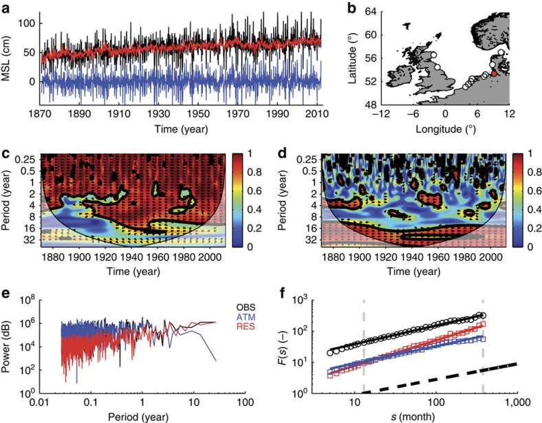
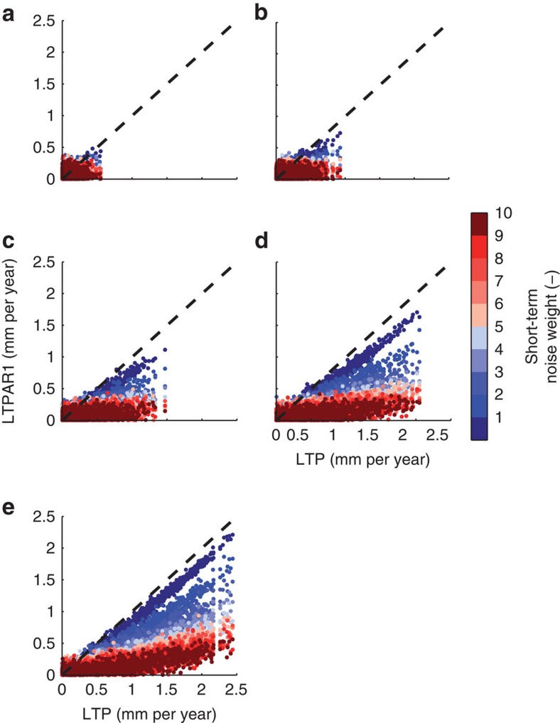
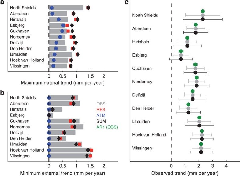
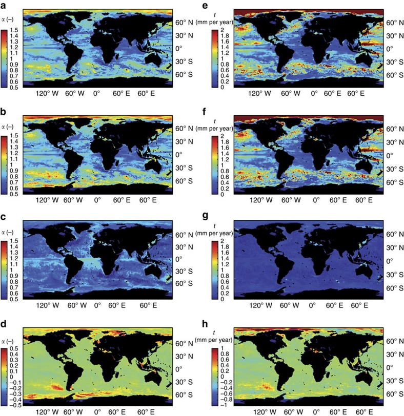
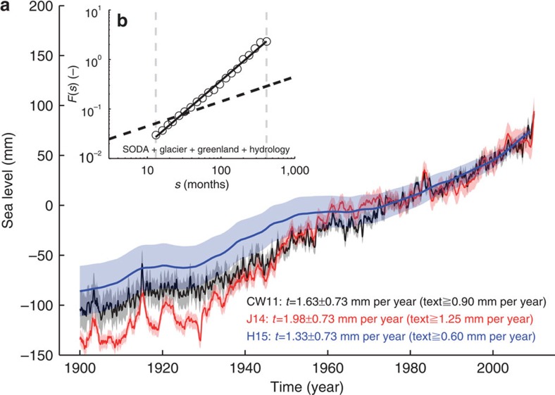
While there is scientific consensus that global and local mean sea level (GMSL and LMSL) has risen since the late nineteenth century, the relative contribution of natural and anthropogenic forcing remains unclear. Here we provide a probabilistic upper range of long-term persistent natural GMSL/LMSL variability (P=0.99), which in turn, determines the minimum/maximum anthropogenic contribution since 1900. To account for different spectral characteristics of various contributing processes, we separate LMSL into two components: a slowly varying volumetric component and a more rapidly changing atmospheric component. We find that the persistence of slow natural volumetric changes is underestimated in records where transient atmospheric processes dominate the spectrum. This leads to a local underestimation of possible natural trends of up to ∼1 mm per year erroneously enhancing the significance of anthropogenic footprints. The GMSL, however, remains unaffected by such biases. On the basis of a model assessment of the separate components, we conclude that it is virtually certain (P=0.99) that at least 45% of the observed increase in GMSL is of anthropogenic origin.

Figure 1. Spectral properties of LMSL and its components.

(a) Time series of OBS (black), ATM (blue) and RES (red) at the tide gauge of Cuxhaven over the period from 1871 to 2011. The location of the tide gauges is shown in (b) with Cuxhaven marked in red. Wavelet coherence plots (Morlet wavelet) of ATM and RES versus OBS are shown in (c,d). The black lines show the 5% significance level using the red noise model. The corresponding global power spectra for OBS, ATM and RES inferred from a fast Fourier transformation are shown in (e,f). Fluctuation functions estimated with DFA2 for OBS, ATM and RES, respectively. The grey dotted lines mark the time window (13≤s≤423 months) for which the Hurst exponents α were estimated. The black dotted line marks a Hurst exponent α of 0.5, that is, uncorrelated noise.

Figure 2. The effect of AR1 noise on modelling natural and external trends in LMSL.

(a–e) Natural trends in long-term correlated Gaussian data (LTP; 1,000 time series with a length of 1,692 months) versus natural trends in long-term correlated Gaussian data with additive AR1 noise (LTPAR1). The different colour shades correspond to the weight with which the AR1 noise was added to the long-term correlated data (1–10 times larger than the s.d. of the purely long-term correlated Gaussian data; in the North Sea the s.d. of the ATM exceeds that of the RES by 1–3 times). The natural trends correspond to a time series with a unit s.d. of 10 cm in the combined time series (which is roughly the median in the analysed North Sea records). Simulation results are shown for long-term correlated Gaussian data with (a) α=0.6, (b) α=0.7, (c) α=0.8, (d) α=0.9 and (e) α=1.0. For the lag-1 autocorrelation a value of c=0.1, which is the maximum value obtained from the ATM, has been applied.

Figure 3. Maximum natural and minimum/maximum external trends in LMSL at tide gauges in the North Sea.

(a) Maximum natural trends (P=0.99) derived by the method from refs , , for Hurst exponents α estimated with OBS (grey bars), ATM (blue dots), RES (red squares) and the root sum of squares of ATM and RES (SUM, black diamonds) over the period from 1900 to 2011. The corresponding minimum external trends, calculated as the difference between the observed and maximum natural trends, are shown in (b). In (c) the observed trends are shown in its classical expression with their lower and upper 99% confidence bounds (that is, the minimum and maximum external contribution, see also Methods) obtained from OBS (grey) and SUM (black). For comparison also the results for a classical AR1 model are shown (green). Note that the observed trends still contain vertical land motions, which are responsible for the vast majority of the differences obtained between the different stations.

Figure 4. Hurst exponents α and maximum natural centennial trends in modelled LMSLsyn.

(a–c) α values as calculated for different components of LMSLsyn, RESsyn and OBPsyn over the period from 1899 to 2008. (d) Differences between the α values from LMSLsyn and RESsyn. (e–g) Maximum natural trends (P=0.99) for LMSLsyn, RESsyn and OBPsyn fields under the assumption of a short-term (α=0.5) or a long-term correlated (α>0.5) process. (h) Differences between maximum natural trends in sea level derived from an integrated assessment of LMSLsyn minus the root sum of squares of natural trends calculated for OBPsyn and RESsyn separately.

Figure 5. Maximum natural and minimum external trends in GMSL.

(a) Shown are three recent reconstructions of GMSL based on CW11 (ref. 2), J14 (ref. 3) and H15 (ref. 4) over the period 1900–2009. The shadings show their 1σ uncertainties. Their linear trends are given in the legend. All reconstructions suffer, with respect to their temporal variability, from sampling problems related to the temporally and spatially unevenly distributed location of tide gauge measurements. Therefore, the temporal GMSL variability and the resulting naturally forced centennial trends (P=0.99) have been assessed using spatial average of the LMSLsyn fields (SSH, glacier, Greenland ice sheet and hydrology), which are available over the entire global ocean over the period from 1871 to 2008. The resulting fluctuation function derived from a DFA2 is shown in (b). The fluctuation function yields an α value of 1.28. Following the approach described in refs , , , this implies an upper bound of naturally forced centennial trends (1900–2009) of 0.73 mm per year (P=0.99). This suggests that the observed twentieth century GMSL rise is already outside the range of natural variability with a minimum external contribution (dependent on the reconstruction) of 0.60–1.25 mm per year (P=0.99).

References

1. Church J. A. et al.. in Climate Change 2013: The Physical Science Basis. Contribution of Working Group I to the Fifth Assessment Report of the Intergovernmental Panel on Climate Change Cambridge University Press (2013) .
1. Church J. A. & White N. J. Sea-level rise from the late 19th to the early 21st century. Surv. Geophys. 32, 585–602 (2011) .
1. Jevrejeva S., Moore J. C., Grinsted A. & Woodworth P. L. Recent global sea level acceleration started over 200 years ago? Geophys. Res. Lett. 35, L08715 (2008) .
1. Hay C. C., Morrow E., Kopp R. E. & Mitrovica J. X. Probabilistic reanalysis of twentieth-century sea-level rise. Nature 517, 481–484 (2015) . - PubMed
1. Kemp A. C. et al.. Climate related sea-level variations over the past two millennia. Proc. Natl Acad. Sci. USA 105, 13252–13257 (2011) . - PMC - PubMed
Publication types
LinkOut - more resources