Non-parametric representation and prediction of single- and multi-shell diffusion-weighted MRI data using Gaussian processes

Abstract

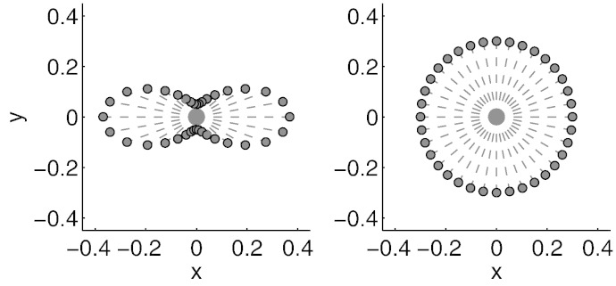
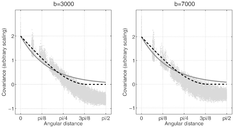
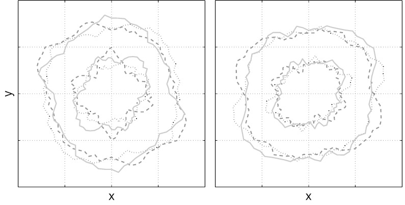
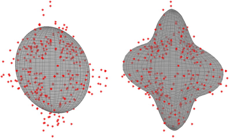
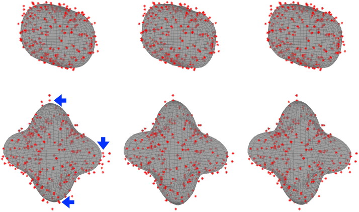
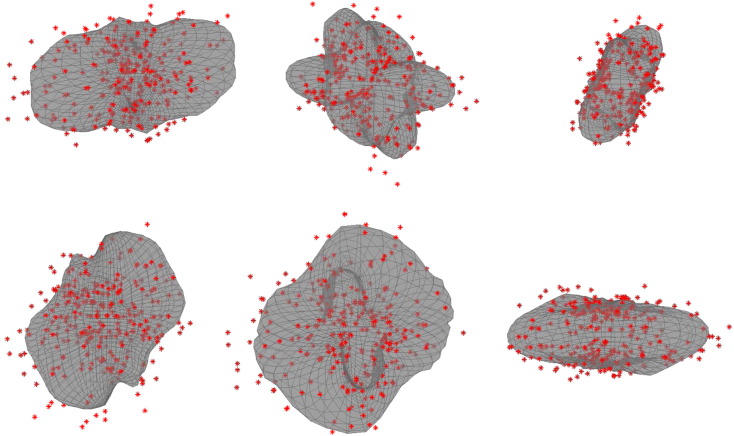
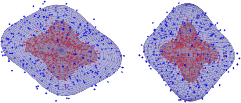
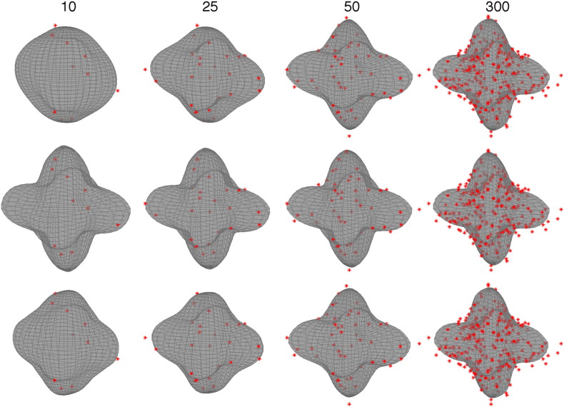
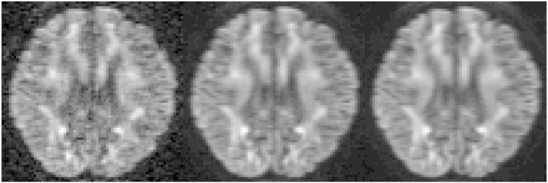
Diffusion MRI offers great potential in studying the human brain microstructure and connectivity. However, diffusion images are marred by technical problems, such as image distortions and spurious signal loss. Correcting for these problems is non-trivial and relies on having a mechanism that predicts what to expect. In this paper we describe a novel way to represent and make predictions about diffusion MRI data. It is based on a Gaussian process on one or several spheres similar to the Geostatistical method of "Kriging". We present a choice of covariance function that allows us to accurately predict the signal even from voxels with complex fibre patterns. For multi-shell data (multiple non-zero b-values) the covariance function extends across the shells which means that data from one shell is used when making predictions for another shell.

Keywords: Diffusion MRI; Gaussian process; Multi-shell; Non-parametric representation.

Fig. 1

Simulated (2D) examples of diffusion weighted measurements. The direction along which diffusion weighting was applied is shown by a dashed line and the measured signal along that direction is indicated by the distance of the round marker from the origin. The left panel shows the case where diffusivity is three times greater along the y-axis than along the x-axis. The right panel demonstrates the case where diffusivity is equal in all directions. The extension of this to 3D is straightforward, though a little tricky to demonstrate in a figure. If we extend the figure in the left panel to 3D and assume that the diffusivity along the direction perpendicular to the paper is the same as for the x-direction, the points sampled on the resulting surface would form a “red blood cell” seen from the side. Correspondingly in the right panel if we assume equal diffusivity in all three directions the resulting surface would be a sphere.

Fig. 2

The empirically observed covariance versus angle between diffusion weighting directions (b-vectors) for the HCP b = 3000 (left) and b = 7000 data sets described in Table 1. Each point represents one pair of b-vectors and the covariance is calculated across all intra-cerebral voxels. The points with zero angle corresponds to the variance (pooled across all voxels) for each direction. The solid grey line corresponds to the exponential (Eq. (9)) and the dashed black line to the spherical (Eq. (10)) covariance function. These are “Chi-by-eye” lines and are there to demonstrate their respective general appearance in relation to the empirically observed covariance. The same “length scale” parameters were used for both plots (a = 1.23 and a = 0.5 for the spherical and the exponential functions respectively).

Fig. 3

Examples of prior shapes (cut at arbitrary plane) generated using hyperparameters estimated from the HCP b = 1500 data (outer shell) and the HCP b = 5000 (inner shell). The solid, dashed and dotted shapes represent three different realisations drawn from the distribution of possible shapes. On the left hand side the priors were drawn independently for the two shells and on the right they were drawn from the multi-shell model (Eq. (16)). Note how in the absence of data, the expected shape is approximately spherical (isotropic diffusion) and that the (relative) variability is greater for the inner shell. Note also that for the multi-shell model (right hand size) the shapes covary across the shells.

Fig. 4

Example of predictions from a tensor fit (left) panel and from a Gaussian process fit (right) panel to a crossing fibre voxel in the Centrum Semiovale in the region where the superior longitudinal fasciculus II crosses the corticospinal tract. The data is a single shell with a b-value of 3000. The data is shown as red dots and the model prediction as a grey surface. As expected the Gaussian process shows a much better ability to predict the data from such voxels despite being even faster to calculate than the tensor prediction.

Fig. 5

The top row shows the signal (with a b-value of 3000) from a cortical grey matter voxel and the bottom row from a white matter voxel with a three-way crossing. The left most column shows data and predictions obtained when deriving the hyperparameters from the grey matter voxel, the middle column when deriving them from the white matter voxel and the right most column when deriving them jointly from both voxels. It can be seen (lower left sub-figure) that the modelling of the white matter voxel is affected somewhat negatively when using the hyperparameters estimated from the grey matter voxel. The arrows point to data points where it can be seen that the distance to the model fit is greater than for the other two columns. When using the jointly derived hyperparameters, the $\mathcal{G}\mathcal{P}$ (lower right sub-figure) manages to capture the features of the data equally well as when the white matter derived hyperparameters are used (lower middle sub-figure).

Fig. 6

The figure shows data (red) and Gaussian process ($\mathcal{G}\mathcal{P}$) fit (grey) from a b = 7000 shell from the pilot phase of the HCP. The six panels correspond to six randomly selected voxels in a transversal slice at the level of the Centrum Semiovale. The hyperparameters for the $\mathcal{G}\mathcal{P}$ was the same for all voxels (and calculated from a random selection of 1000 intracerebral voxels). It can be seen that the $\mathcal{G}\mathcal{P}$ has been able to successfully model the signal from the six voxels despite exhibiting vastly different signal profiles. It can for example be appreciated from the signal that the top panel in the middle column corresponds to a three-way crossing fibre, the top panel in the right column a two-way crossing fibre and the lower panel in the middle column a single (dominating) fibre. The top-left and bottom-right panels correspond to grey matter voxels.

Fig. 7

Example of multi-shell predictions. The same voxel as in Fig. 4 but using two other shells with b-values of 1500 (blue) and 5000 (red). Both panels show the same data rotated to demonstrate it more fully. In the multi-shell model the data from one shell will impact on the predictions about the other shell and yet it is clear from this figure that the predictions for the high b-value shell has additional detail and is not just a scaled version of the lower b-value predictions.

Fig. 8

This figure demonstrates the predictions for a b = 5000 voxel when considering only the b = 5000 data points (top row) or when using also the b = 3000 data (middle row) or the b = 1500 data (bottom row). The predictions are shown when using only the first 10, 25 and 50 points from a set of 300 as well as when using all 300 points. It can be seen (middle row) that the ability to make meaningful predictions from a paucity of data is very much improved when utilising information from the neighbouring shell (b = 3000). It can also be seen (bottom row) that when the “supporting shell” is further away, its impact is smaller, but still appreciable when the number of data points is 25 or less.

Fig. 9

Examples of observed and predicted images for the single shell model. The left panel shows an image acquired with a b-value of 3000 and the diffusion gradient [1 0 0], the middle panel shows the Gaussian process prediction when the observed image was part of the training data (smoothing) and the right panel when the observed image was not (interpolation).

References

1. Aganj I., Lenglet C., Sapiro G., Yacoub E., Ugurbil K., Harel N. Reconstruction of the orientation distribution function in single and multiple-shell q-ball imaging within constant solid angle. Magn. Reson. Med. 2010;640(2):554–566. - PMC - PubMed
1. Alexander A.L., Wu Y.-C., Venkat P.C. Hybrid diffusion imaging (HYDI) Magn. Reson. Med. 2006;380(2):1016–1021. - PubMed
1. Andersson J.L.R., Skare S. A model-based method for retrospective correction of geometric distortions in diffusion-weighted EPI. NeuroImage. 2002;16:177–199. - PubMed
1. Andersson J.L.R., Skare S. Chapter 17: image distortion and its correction in diffusion MRI. In: Jones D.K., editor. Diffusion MRI: Theory, Methods, and Applications. Oxford University Press; Oxford, United Kingdom: 2011. pp. 285–302.
1. Andersson J.L.R., Sotiropoulos S. Joint Annual Meeting ISMRM-ESMRMB. 2014. A gaussian process based method for detecting and correcting dropout in diffusion imaging; p. 2567.