Spatially-global integration of closed, fragmented contours by finding the shortest-path in a log-polar representation

Abstract

Finding the occluding contours of objects in real 2D retinal images of natural 3D scenes is done by determining, which contour fragments are relevant, and the order in which they should be connected. We developed a model that finds the closed contour represented in the image by solving a shortest path problem that uses a log-polar representation of the image; the kind of representation known to exist in area V1 of the primate cortex. The shortest path in a log-polar representation favors the smooth, convex and closed contours in the retinal image that have the smallest number of gaps. This approach is practical because finding a globally-optimal solution to a shortest path problem is computationally easy. Our model was tested in four psychophysical experiments. In the first two experiments, the subject was presented with a fragmented convex or concave polygon target among a large number of unrelated pieces of contour (distracters). The density of these pieces of contour was uniform all over the screen to minimize spatially-local cues. The orientation of each target contour fragment was randomly perturbed by varying the levels of jitter. Subjects drew a closed contour that represented the target's contour on a screen. The subjects' performance was nearly perfect when the jitter-level was low. Their performance deteriorated as jitter-levels were increased. The performance of our model was very similar to our subjects'. In two subsequent experiments, the subject was asked to discriminate a briefly-presented egg-shaped object while maintaining fixation at several different positions relative to the closed contour of the shape. The subject's discrimination performance was affected by the fixation position in much the same way as the model's.

Keywords: Closed contour; Figure Ground Organization; Log-polar representation; Shortest path.

Figure 1

A camera image of a rocking horse on a textured floor (left) and the canny edges of the scene (right).

Figure 2

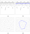
The procedure for generating a target stimulus with a concave polygon. (a) Ten random points were connected by using a Traveling Salesman Problem tour that resulted in a concave polygon. (b) This polygon was fragmented into pieces with equal lengths of 30 pixels and with similar gaps. (c) The remaining windows were filled with noise line segments. In the experiment, the contrast was opposite to the images shown in this paper, i.e., the line stimuli were white on black.

Figure 3

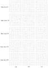
Sample stimuli consisting of convex polygons. Each row contains 3 different polygons with the level of average jitter increasing from top to bottom. Note how hard it is to see the targets with the two highest jitter levels.

Figure 4

Sample stimuli of concave polygons. See the caption of Figure 3 for details.

Figure 5

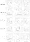
Contours drawn by the 3 subjects with the stimuli shown in Figure 3a. Note the high degree of consistency among them at the lowest jitter levels.

Figure 6

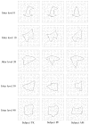
Contours drawn by the 3 subjects for the stimuli in Figure 4a. Note that there is good consistency among the subjects at the two lowest jitter levels.

Figure 7

(a) One subject’s constructed curve. (b) The same image with its line segments thickened to facilitate computing P_CD. Red indicates contour segments selected correctly. Green indicates noise segments included in the constructed curve.

Figure 8

The average P_CD for convex and concave polygons in Experiment 1. Error bars are standard errors of the mean.

Figure 9

P_CD averaged across the 3 subjects for both convex and concave polygons. Standard Errors are estimated from the 3 measurements corresponding to the individual results shown in Figure 8.

Figure 10

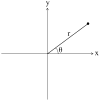
Cartesian (x,y) and polar (r,θ) coordinate systems.

Figure 11

The stimulus on the retina and the representation in area V1 of the macaque monkey’s brain. (A) The polar web pattern that stimulated the visual system of a monkey treated with radioactively labeled glucose. (B) After accumulating the tracer in the most active cells, the radiograph of the monkey’s area V1 was made as a nearly rectilinear grid. From “Deoxyglucose Analysis of Retinotopic Organization in Primate Striate Cortex,” by R. B. H. Tootell, M. S. Silverman, E. Switkes, & R. L. DeValois, 1982, Science, 218, p. 902. Copyright 1982 by the American Association for the Advancement of Science.

Figure 12

An idealized log-polar mapping. Circles on the retina with proportionally increasing radii are mapped to equally-spaced horizontal lines in the log-polar representation (see the green, blue and brown lines, marked as 1, 2, and 3). The straight lines that go through the center of the retina are mapped to the vertical lines in the log-polar representation (see the red and pink lines, marked as 4 and 5). Note that the negative part of the x-axis on the retina is represented twice at θ = −π and at +π in the log polar map (see the yellow lines, marked as 6). This is the only line with such a property. It is implied by the log-polar mapping because a closed circle is transformed into an open line segment.

Figure 13

Four squares on the retina (a) are transformed into curves in the log-polar representation (b). Note that the right angles in the retina are transformed to right angles in log-polar representation. The three squares whose centers coincide with the center of the retina (red, blue and green) are represented by identical curves in the log-polar coordinates except for translation along the horizontal or vertical axis. The log-polar representation of the pink square, which is shifted to the right, is different. This represents the fact that the log-polar representation is sensitive (not invariant) to even small translations on the retina. It turns out, however, that the shortest path computed in the log-polar representation is not very sensitive to such small translations on the retina.

Figure 14

Model SP. The image in the Cartesian coordinates (c) was transformed to the image in the log-polar coordinates (a). The model used the designated starting point. It found the path shown in (b) that minimized the cost. After this path was found, it was transformed back to Cartesian coordinates (d). Note that edges close to the fixation point in the retinal image project to long segments in the log-polar representation and segments that are far from the center of the image project to very short segments in the log-polar representation.

Figure 15

Model LI-SP. (a) is a log polar representation of the image shown in (d). The image in (d) was subjected to the linear interpolation operation. The result is shown in (e). The image in (e) was transformed to the log-polar representation (b). By using the shortest path algorithm from the designated starting point, the shortest path was found. After the path was found, it was back transformed to the Cartesian coordinate (f).

Figure 16

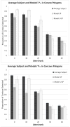
The average subject and the two models’ (SP & LI-SP) P_CD for the convex and the concave polygons.

Figure 17

The average P_CD of the three subjects for the convex and the concave polygons in Experiment 2. Error bars are standard errors of the mean.

Figure 17

The average P_CD of the three subjects for the convex and the concave polygons in Experiment 2. Error bars are standard errors of the mean.

Figure 18

The average subject’s and the model LI-SP-EST’s P_CD for the convex and the concave polygons in Experiment 2.

Figure 18

The average subject’s and the model LI-SP-EST’s P_CD for the convex and the concave polygons in Experiment 2.

Figure 19

The four types of egg stimuli used in this experiment. Dense sampling is shown on the left and sparse sampling on the right. Large eggs are in top row and small eggs are in the bottom row. The contrast was reversed in the actual experiment.

Figure 20

Results obtained in 4 sessions with egg stimuli. The ordinate shows d′, and the abscissa shows either large eggs around the fixation point or small eggs above or below the fixation point. The two bars indicate the two types of sampling. Error bars represent the standard errors calculated from each session.

Figure 21

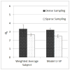
Comparison of the results of our average subject with the model for the eggs around the center. Error bars of the average subject represent the standard errors calculated from the four subjects. Error bars of the model represent the standard errors calculated from the each session.

Figure 22

The center of the egg was located in one of four regions: small circle or 3 annuli.

Figure 23

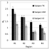
Performance of the subjects when the fixation point was inside the egg. The fixation point was located in one of the four regions inside the egg. R1 is the region around the fixation point and R4 is the region around the boundary of the curve. See the Procedure for more details.

Figure 24

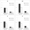
Comparison of our average subject and the model when the fixation point is inside the eggs.

References

1. Anstis SM. A chart demonstrating variations in acuity with retinal position. Vision Research. 1974;14(7):589–592. - PubMed
1. Ben-Shahar O, Ben-Yosef G. Tangent bundle elastica and computer vision. IEEE Transactions on Pattern Analysis and Machine Intelligence. 2015;37:161–174. - PubMed
1. Ben-Yosef G, Ben-Shahar O. A tangent bundle theory for visual curve completion. IEEE Transactions on Pattern Analysis and Machine Intelligence. 2012;34:1263–1280. - PubMed
1. Bertamini M. The importance of being convex: An advantage for convexity when judging position. Perception. 2001;30(11):1295–1310. - PubMed
1. Bertamini M, Wagemans J. Processing convexity and concavity along a 2-D contour: figure-ground, structural shape, and attention. Psychonomic Bulletin & Review. 2013;20(2):191–207. - PubMed
Publication types