A frequency-dependent decoding mechanism for axonal length sensing

Abstract

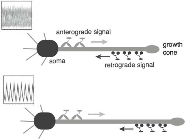
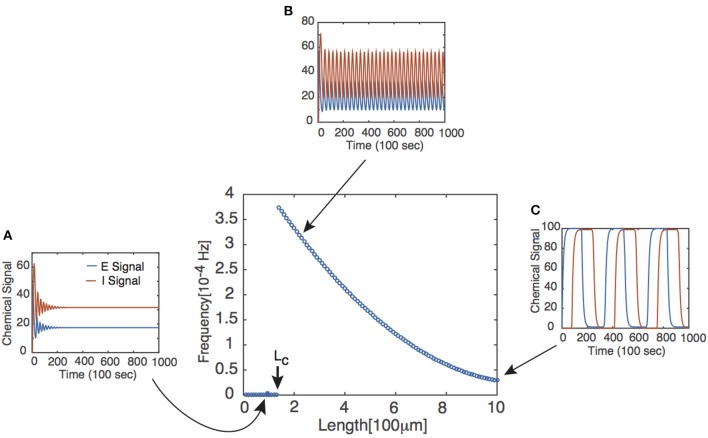
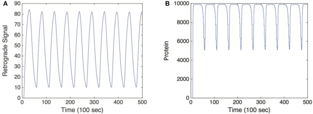
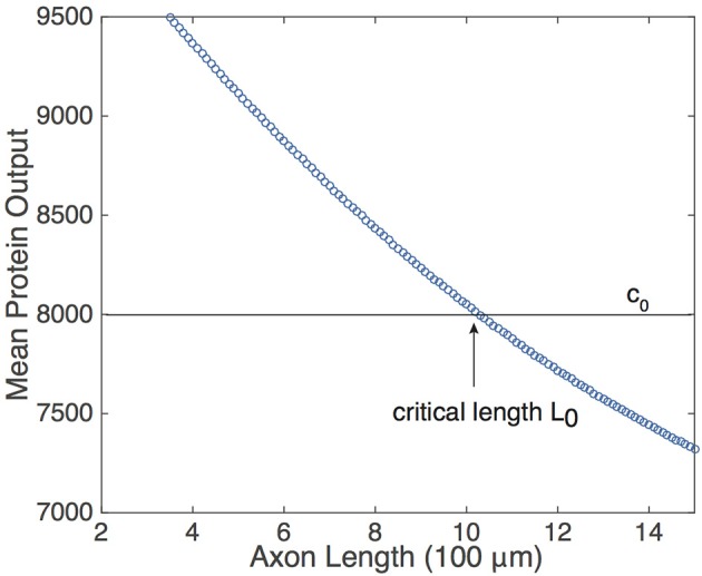
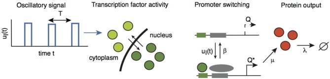
We have recently developed a mathematical model of axonal length sensing in which a system of delay differential equations describe a chemical signaling network. We showed that chemical oscillations emerge due to delayed negative feedback via a Hopf bifurcation, resulting in a frequency that is a monotonically decreasing function of axonal length. In this paper, we explore how frequency-encoding of axonal length can be decoded by a frequency-modulated gene network. If the protein output were thresholded, then this could provide a mechanism for axonal length control. We analyze the robustness of such a mechanism in the presence of intrinsic noise due to finite copy numbers within the gene network.

Keywords: axonal length control; biochemical oscillations; frequency decoding; gene network; intrinsic noise; protein thresholds.

Figure 1

Schematic diagram of the bidirectional motor-transport mechanism for axonal length sensing hypothesized by Rishal et al. (2012). A kinesin-based anterograde signal activates a dynein-based retrograde signal that itself represses the anterograde signal via negative feedback. The frequency of the resulting oscillatory retrograde signal decreases with axonal growth.

Figure 2

Frequency of periodic solutions plotted against axonal length. [Plot was obtained by looking at the power spectrum of the retrograde signal and taking the frequency of the signal to be where the sharp peak of the spectrum occurred.] Insets show time series plots at specific values of the delay generated using the dde23 program in MATLAB: (A) τ = 1, (B) τ = 2, (C) τ = 10. Other parameter values are n = 4, I₀ = 10, W_E = W_I = 9.5 such that τ_c ≈ 1.5.

Figure 3

Simulation of the feed forward serial network Equation (5) in response to a retrograde signal from Equation (2). (A) Retrograde signal being fed into gene network, τ = 5. (B) Convergence of the solutions of Equation (5) to a T-periodic solution post transience. h[u] is taken to be the same function as f[u] defined in Equation (3) multiplied by a factor of 1000, and we set λ = 0.01. Other parameter values are as in Figure 2.

Figure 4

Relationship of the mean protein output $\overline{c}$ and axonal length L, obtained by time averaging the solution to Equation (5) for several values of τ. Function definitions and parameter values are as in Figures 2, 4. The existence of a threshold protein output c₀ could provide a mechanism for determining a critical length L₀.

Figure 5

A gene promoter driven by the oscillatory retrograde signal u_I(t). Adapted and redrawn from Tostevin et al. (2012).

Figure 6

Plot of mean protein output $\overline{c}$ vs. axonal length L. Results are based on simulations of the chemical master Equation (14) using the Gillespie algorithm with input s(t) = h[u_I(t)]. Parameter values used to generate retrograde signal u_I(t) are the same as in Figure 2. Other parameter values are β = 1, μ = 0.1, λ = 0.01, and N = 1000.

Figure 7

Schematic diagram illustrating how the presence of noise in the protein output leads to an uncertainty ΔL in the critical axonal length L₀ at which the threshold is crossed. An analogous result applies to decoding of protein concentration gradients.

Figure 8

Plot of estimated errors in axonal length based on 100 simulations of the chemical master Equation (14) using the Gillespie algorithm with input s(t) = h[u_I(t)]. (A) Plot of uncertainty in axonal length ΔL vs. threshold axonal lengths L₀. (B) Relative error (ΔL ∕ L₀) vs. axonal length. Same parameters as Figure 6. L₀ was found by averaging over the mean protein outputs and determining what length that protein value corresponded to according to the curve shown in Figure 4. ΔL was determined by looking at what axonal length each individual mean protein output realization corresponded to according to Equation (4) and then finding the variance in this set of values.

References

1. Brown K. M., Gillette T. A., Ascoli G. A. (2008). Quantifying neuronal size: summing up trees and splitting the branch difference. Semin. Cell Dev. Biol. 19, 485–493. 10.1016/j.semcdb.2008.08.005 - DOI - PMC - PubMed
1. Cai L., Dalal C. K., Elowitz M. B. (2008). Frequency-modulated nuclear localization bursts coordinate gene regulation. Nature 45, 485–491. 10.1038/nature07292 - DOI - PMC - PubMed
1. Gardner T. S., Cantor C. R., Collins J. J. (2000). Construction of a genetic toggle switch in e. coli. Nature 403, 339–342. 10.1038/35002131 - DOI - PubMed
1. Goslin K., Banker G. (1989). Experimental observations on the development of polarity by hippocampal neurons in culture. J. Cell Biol. 108, 1507–1516. 10.1083/jcb.108.4.1507 - DOI - PMC - PubMed
1. Howard M. (2012). How to build a robust intracellular concentration gradient. Trends Cell Biol. 22, 311–317. 10.1016/j.tcb.2012.03.002 - DOI - PubMed
LinkOut - more resources