Fast, Continuous Audiogram Estimation Using Machine Learning

Abstract

Objectives: Pure-tone audiometry has been a staple of hearing assessments for decades. Many different procedures have been proposed for measuring thresholds with pure tones by systematically manipulating intensity one frequency at a time until a discrete threshold function is determined. The authors have developed a novel nonparametric approach for estimating a continuous threshold audiogram using Bayesian estimation and machine learning classification. The objective of this study was to assess the accuracy and reliability of this new method relative to a commonly used threshold measurement technique.

Design: The authors performed air conduction pure-tone audiometry on 21 participants between the ages of 18 and 90 years with varying degrees of hearing ability. Two repetitions of automated machine learning audiogram estimation and one repetition of conventional modified Hughson-Westlake ascending-descending audiogram estimation were acquired by an audiologist. The estimated hearing thresholds of these two techniques were compared at standard audiogram frequencies (i.e., 0.25, 0.5, 1, 2, 4, 8 kHz).

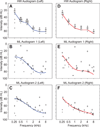
Results: The two threshold estimate methods delivered very similar estimates at standard audiogram frequencies. Specifically, the mean absolute difference between estimates was 4.16 ± 3.76 dB HL. The mean absolute difference between repeated measurements of the new machine learning procedure was 4.51 ± 4.45 dB HL. These values compare favorably with those of other threshold audiogram estimation procedures. Furthermore, the machine learning method generated threshold estimates from significantly fewer samples than the modified Hughson-Westlake procedure while returning a continuous threshold estimate as a function of frequency.

Conclusions: The new machine learning audiogram estimation technique produces continuous threshold audiogram estimates accurately, reliably, and efficiently, making it a strong candidate for widespread application in clinical and research audiometry.

Figure 1

Illustration of the sampling algorithm used by the Gaussian process (GP) for machine learning (ML) audiogram estimation. (A) Posterior mean is computed by the GP using the sampled points. Red diamonds indicate the tone was inaudible; blue pluses, audible. (B) Posterior variance is computed by the GP using the sampled points, and the point of maximum variance is identified (purple star). (C) The point of maximal variance is queried for listener audibility (black arrow). Once it is determined that the listener did not hear this tone, the updated set of points is used by the GP to re-compute the posterior mean with a more elevated threshold near the frequency of that tone.

Figure 2

Sample plots of left- and right-ear audiograms obtained and samples conducted for a representative listener (Listener 4) using the manual HW technique (A, D), the first run of the ML algorithm (B, E), and the second run of the ML algorithm (C, F). Marks represent the frequencies and intensities of the stimuli that were presented, with pluses denoting listener detections and diamonds denoting misses. The superimposed curves are the final audiogram estimates produced by each technique. Note that the small displacements along the frequency axis in (A) and (B) only are to make repeat stimuli more visible and do not reflect actual deviations in the frequency of presented tones.

Figure 3

Sample plots of ML audiogram results for (A) an ear with relatively normal hearing; (B) an ear with sloping high-frequency hearing loss; and (C) an ear with a no-response at 8000 Hz. “X” and “O” marks denote values estimated from the manual HW audiogram (connected by straight lines). The superimposed curves show the results from the automated ML audiogram.

Figure 4

Cumulative agreement between automated ML and manual HW audiograms as a function of GP algorithm iteration. Mean absolute difference was calculated by obtaining the current ML estimate of the threshold audiogram at each iteration during one run, then calculating the absolute difference between that estimate and the HW threshold audiogram, averaged across all 6 audiogram frequencies. (A) and (B) show examples for two ears (Listener 4, the same listener as in Figure 2), and (C) shows this trend averaged across all runs where the ML audiograms terminated at 36 iterations (53 of 80 runs). Blank areas denote points at which the ML procedure did not produce a posterior mean with a clear boundary, so error could not be assessed (but in practice is very high). Gray shading on (C) indicates ±1 standard deviation from the mean.

Figure 5

Normalized posterior variance as a function of algorithm iteration. Normalized posterior variance was calculated by dividing the sum all values in the variance function at each iteration by the total size of the variance function matrix. (A) and (B) show examples for two ears (Listener 4, the same listener as in Figure 2), and (C) shows this trend averaged across all listeners whose ML audiograms terminated at 36 iterations. Gray shading on (C) indicates ±1 standard deviation from the mean.

Figure 6

Data from Listener 17, who fell asleep while the ML audiogram estimation was underway. (A) The final ML audiogram from one ear, superimposed upon the HW audiogram obtained for the same ear (“X”). (B) Samples collected while conducting the ML audiogram. Note the inconsistency in responses, with detections and misses in very close proximity. (C) Plot of normalized posterior variance as a function of iteration for this listener. This listener reached the ceiling on the number of allowable iterations for this ear, 64. Unlike the variance trends in Figure 5, the variance in this ear actually begins to increase after approximately iteration 15 and remains high even after 64 iterations.

References

-
- American National Standards Institute. Methods for manual pure-tone threshold audiometry. ANSI. 2004;3:21.
- American Speech-Language-Hearing Association. Guidelines for manual pure-tone threshold audiometry. 2005
- Amitay S, Hawkey DJ, Moore DR. Auditory frequency discrimination learning is affected by stimulus variability. Percept Psychophys. 2005;67:691–698. - PubMed
- Békésy GV. A new audiometer. Acta Oto-Laryngologica. 1947;35:411–422.
- Berliner JE, Durlach NI. Intensity perception. IV. Resolution in roving-level discrimination. J Acoust Soc Am. 1973;53:1270–1287. - PubMed
Publication types
MeSH terms
Grants and funding
LinkOut - more resources
Full Text Sources
Miscellaneous