Whole-central nervous system functional imaging in larval Drosophila

Abstract

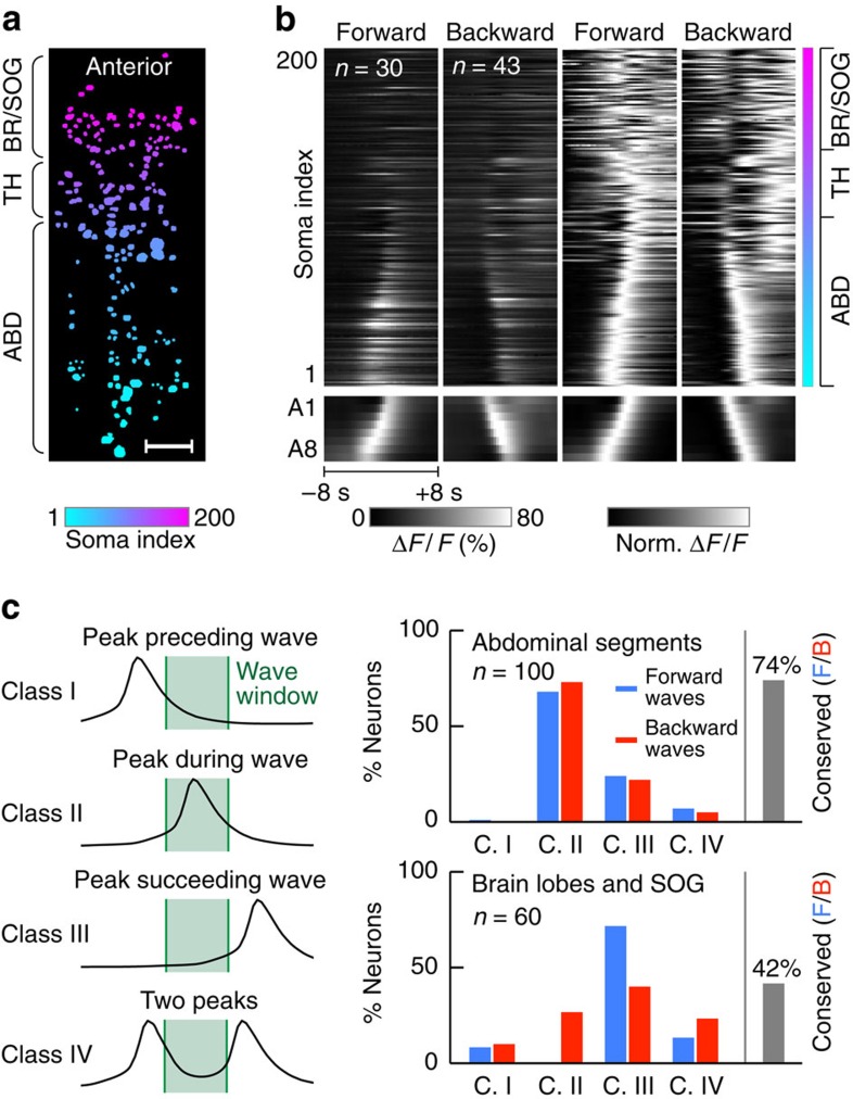
Understanding how the brain works in tight concert with the rest of the central nervous system (CNS) hinges upon knowledge of coordinated activity patterns across the whole CNS. We present a method for measuring activity in an entire, non-transparent CNS with high spatiotemporal resolution. We combine a light-sheet microscope capable of simultaneous multi-view imaging at volumetric speeds 25-fold faster than the state-of-the-art, a whole-CNS imaging assay for the isolated Drosophila larval CNS and a computational framework for analysing multi-view, whole-CNS calcium imaging data. We image both brain and ventral nerve cord, covering the entire CNS at 2 or 5 Hz with two- or one-photon excitation, respectively. By mapping network activity during fictive behaviours and quantitatively comparing high-resolution whole-CNS activity maps across individuals, we predict functional connections between CNS regions and reveal neurons in the brain that identify type and temporal state of motor programs executed in the ventral nerve cord.

Figure 1. Light-sheet microscopy and computational tools for whole-CNS functional imaging.

(a) For optimal optical access, the CNS of a Drosophila third (3rd) instar larva is extracted by surgery and embedded in a soft, transparent agarose cylinder supported by a glass capillary for mounting in the hs-SiMView light-sheet microscope. (b) The CNS explant is then transferred to the microscope's specimen chamber filled with physiological saline. The illustration shows the hs-SiMView microscope core for SiMView functional imaging, including the central specimen chamber, two illumination objectives for bi-directional fluorescence excitation with scanned laser light sheets and two opposing detection objectives mounted on high-speed piezo stages. The 3D volumes covered by the two piezo-operated detection objectives are matched with a precision of a few micrometres using custom Y-Z-θ fine adjustment stages and objective X-flexures. (c) In conventional multi-view light-sheet microscopy, the specimen is physically moved through the light sheet for volumetric imaging, which fundamentally constrains imaging speed. In contrast, high-speed multi-view volumetric imaging in hs-SiMView is achieved by keeping the specimen stationary and instead co-translating the focal planes of the two opposing detection systems using piezos. Simultaneously, the thin specimen volume at the location of the focal planes is illuminated bi-directionally with light sheets translated by spatiotemporally matched laser scanning. (d) Using a custom processing pipeline for hs-SiMView functional imaging data, the geometry of the specimen is automatically determined from multi-view image data, image foreground is stored using lossless compression in a custom block-based file format, multiple camera views are spatially registered, multi-view image data are fused, specimen drift is compensated locally and globally across the time-lapse experiment, and a ΔF/F representation of the hs-SiMView time-lapse data set is computed. Using a custom data analysis pipeline, locomotor activity patterns are automatically detected and classified, and high-resolution computational maps of CNS-wide activity timing are constructed for multiple fictive behaviours. In order to quantitatively compare CNS-wide activity maps across multiple nervous systems, a CNS template is constructed from all data sets and subsequently used to transform all image data into a common reference coordinate system using nonlinear spatial registration.

Figure 2. Whole-CNS functional imaging of the isolated Drosophila larval nervous system.

(a) Whole-CNS functional imaging at 5 Hz of a Drosophila third instar larval CNS expressing 57C10-GAL4,UAS-GCaMP6s, using hs-SiMView light-sheet microscopy. Imaging was performed with one-photon excitation at 488 nm, maintaining a constant imaging speed of 370 frames per second (491 MB per second) for a period of 1 h. Image panels show maximum-intensity projections of ΔF/F (colour look-up-table) and CNS anatomy (grey, gamma-corrected GCaMP6s baseline fluorescence) from dorsal (top) and lateral (bottom) views, for six time points during a backward locomotor sequence. Outline indicates CNS boundary. Longer image sequences from this data set are shown in Supplementary Movies 1 and 2. Complementary data sets recorded with two-photon excitation are shown in Supplementary Movies 3,4,5. (b) Image sequences showing changes in ΔF/F for cell bodies in optical sections taken from ROIs in abdomen (ROIs 1 and 2), thorax (ROI 3) and brain (ROI 4) indicated by white rectangles in panel a. ROI 1 shows an example of rapid changes in ΔF/F across two locomotor waves. ROIs 2–4 show examples of slow changes in ΔF/F across a bout of locomotor waves. Images are median filtered. ABD, abdomen; BL, brain lobes; SOG, suboesophageal ganglion; TH, thorax. Scale bars, 5 μm (b, ROI 1), 10 μm (b, ROIs 2–4) and 50 μm (a).

Figure 3. Fictive locomotion in the Drosophila larval CNS.

(a) Neural activity in all VNC hemisegments was captured using 16 3D ROIs. Segments are labelled as A1–A8 from anterior to posterior. (b) Activity in hemisegments during example locomotor waves (two backward and one forward), shown separately for the left and right sides of the VNC. Traces show ΔF/F. Shading indicates segments A1–A8. (c,d) Average forward (c) and backward (d) waves in a CNS in physiological saline (black: average, light blue: s.e.m.; n=20 waves). The plots show ΔF/F averaged over left and right sides in a representative preparation. (e,f) Same as in c,d, but for an isolated CNS embedded in agarose (n=20 waves), which represents the sample preparation used for imaging with hs-SiMView microscopy. (g,h) Average frequency and duration of forward waves (g) and backward waves (h) in unembedded (NE; n=5 preparations) and embedded preparations (E; n=6 preparations). Error bars show s.d. No significant differences in wave frequency or duration were observed between embedded and unembedded preparations (P≥0.53 for all comparisons, unpaired t-test). (i) Illustration of principles underlying our computational module for automated detection and classification of locomotor waves. Left panels: example backward and forward waves; traces show ΔF/F, with the average response across hemisegments subtracted, to emphasize relative differences. Middle panels: in a 2D space recovered using PCA, locomotor waves are rotations in different directions. Right panels: amplitude (Amp) and phase are computed in the same 2D space; waves are detected as peaks in amplitude and linear ramps in phase. (j) Embedding of all detected waves from one specimen in the 2D space recovered by PCA. Each trace is a wave; left, backward; right, forward. Small black dots indicate wave start times. Scale bar, 25 μm (a).

Figure 4. Mapping whole-CNS activity during locomotor behaviours.

(a) Illustration, for data from one example voxel, of ΔF/F fits performed for purpose of mapping activity timing during locomotor wave windows. Plots show activity traces in all waves sampled (thin, grey), the mean of these traces (black), the rectangular time-based function fit (red) and the flat, time-independent fit (blue). In this example, the time-based fit is much better than the flat fit. This analysis is performed independently for all voxel locations in the image volume. (b,c) Whole-CNS activity timing maps for forward and backward waves (b, dorsoventral slices; c, lateral slices). The statistic shown in a was used to capture relative timing of activity across all detected wave events in one specimen (forward: n=30, backward: n=70). Intuitively, this map shows, for each part for the CNS, the time during locomotor wave windows when activity increases. Arrows in b mark relative progression of locomotor waves on dorsal/ventral sides of the VNC (ascending numbers). Forward and backward wave window sizes were defined as [−10 s, 10 s] and [−6 s, 2 s] (centred on waves in VNC) to ensure wave propagation was captured throughout VNC and overlap of events was avoided. (d) Lateral slices from 3D whole-CNS activity timing map of fictive forward locomotor waves (n=30), with ROIs outlined in white and black (bottom right panel). ROIs include bilaterally symmetrical regions in SOG with increased activity occurring at beginning of forward locomotor waves (1L/R–5L/R), regions in the thorax and at boundary between thorax and abdomen with increased activity occurring during (8L/R–10L/R) or towards the end (6L/R and 7L/R) of forward waves, and regions at dorsal end of brain lobes with increased activity occurring after execution of forward waves (11L/R and 12L/R). (e) ΔF/F traces of ROIs 1L–12L (left two columns) and 1R–12R (right two columns) indicated in panel a, during forward (n=30) and backward (n=66) locomotor waves. Four backward waves were excluded to avoid temporal overlap. For reference, ΔF/F traces of segments A1–A8 in the VNC are shown below data for ROIs 1L/R–12L/R. Dark lines indicate average activity, light areas indicate s.e.m. L, left; R, right; ABD, abdomen; BL, brain lobes; SOG, suboesophageal ganglion; TH, thorax. Scale bars, 50 μm (b–d).

Figure 5. Large-scale profiling of single-neuron activity traces during locomotor behaviours.

(a) Projection of manually annotated 3D somatic ROIs across the CNS used for extracting signals at the single-neuron level (n=200). (b) Neuronal activity, averaged across all detected wave time windows. From left to right: raw ΔF/F for forward waves, raw ΔF/F for backward waves, normalized (Norm.) ΔF/F for forward waves, normalized ΔF/F for backward waves. Greyscale indicates ΔF/F. Matrices above show somatic responses (colour bar to the right indicates location as shown in panel a). Matrices below show corresponding VNC signals (A1–A8, averaged across left and right hemisegments). The global window size was defined as [−8 s, 8 s] (centred on locomotor waves in the VNC) to ensure that wave propagation was captured throughout the VNC, and that comparable statistics were obtained for forward and backward waves without overlap of adjacent event windows. (c) Classification of activity traces of all annotated somas. Left: conceptual illustration of the four classes distinguished in this analysis, including peak activity occurring before wave propagation (defined as the time interval marked by peak activity in abdominal segments A1 and A8, class 1), peak activity occurring during wave propagation (class 2), peak activity occurring after wave propagation (class 3) and two activity peaks separated by a phase of quiescence (defined as a ≥50% reduction in ΔF/F relative to both peaks, class 4). Right: percentages of somas in each class (blue, forward waves; red, backward waves), shown separately for somas in abdominal segments (top) and somas in brain (bottom). Grey bars to the right indicate the percentages of somas with the same classification in forward and backward waves. ABD, abdomen; BR, brain; SOG, suboesophageal ganglion; TH, thorax. Scale bar, 50 μm (a).

Figure 6. Spatial registration of nervous systems.

(a) All CNS explants used for functional imaging expressed GCaMP panneuronally (57C10-GAL4,UAS-GCaMP6s) and tdTomato in anatomically defined regions within the larval CNS (58B03-LexA,LexOP-tdTomato; expression in mushroom bodies and neuropil regions). Columns 1–3 show maximum-intensity projections of unregistered GCaMP images (column 1), spatially registered GCaMP images (column 2) and respective overlays (column 3) for six different Drosophila third instar larval CNS explants. To register nervous systems, we first constructed a CNS template (shown at the bottom of column 2) from GCaMP reference image stacks representing each of the six independent time-lapse experiments (see Methods section). We then registered image data from each experiment to the CNS reference template using nonlinear spatial registration techniques (see Methods section). Overlays of registered image stacks (orange) and CNS reference template (blue) in column 3 show good anatomical correspondence. Since the CNS reference template used for spatial registration of all nervous systems was constructed exclusively from GCaMP images, we used the tdTomato channel (column 4) to evaluate how well an independent expression pattern can be overlaid across multiple nervous system using our registration workflow. In this control analysis, spatial correspondence depends on quality of the spatial registration and biological variability of the expression pattern. Registration of the tdTomato channels of the six explants to the CNS reference template (column 5) resulted in good overlap of expression patterns in CNS 1–5 (column 6), which appeared to highlight the same biological structures in the CNS. The expression pattern in CNS 6 looked qualitatively different from the others, possibly due to transvection of the LexAop-myr::tdTomato transgene. (b) To quantify registration accuracy, two annotators independently determined the 3D positions and relative distances of several CNS landmarks (including landmark locations in abdominal segments and mushroom bodies) in the spatially registered specimens. VNC landmarks were annotated in GCaMP images (obtained by direct registration), whereas brain lobe landmarks were annotated in tdTomato images (indirect registration). The latter measurements thus reflect both accuracy of the registration procedure and biological variability. (c) Inter-annotator agreement of landmark positions independently annotated in the same nervous systems. Scale bar, 50 μm (a).

Figure 7. Neurons in the brain identify type and state of motor programs.

(a) Dorsal (left) and lateral (right) maximum-intensity projections of whole-CNS activity timing map for forward waves (n=30). Colour encodes time point of maximum activity. Luminance encodes improvement in activity fit given time (see Methods section). Top panels show enlarged views of brain/SOG, using a luminance look-up-table restricted to dynamic range of data in this region for better visibility. (b) Top: maximum-intensity projections of eight manually segmented single-soma ROIs from brain/SOG region highlighted in a. Middle and bottom: segmented brain/SOG maps from two additional specimens (CNS 2 and CNS 3), based on 105 and 44 forward waves, respectively. All three nervous systems were spatially co-registered as described in Methods section. Colour code as in a. (c) Overlay of the three brain/SOG segmentation maps shown in b, demonstrating close spatial correspondence of segmented soma locations. Colours indicate specimen identity (green/cyan/magenta: CNS 1/2/3). White circles (xy) and ellipses (xz) in centre of images indicate average accuracy of the spatial registration procedure (inner circle/ellipse: mean, outer circle/ellipse: mean+1 s.d.). Accuracy in brain is 7.8±4.6 μm (mean±s.d., n=60) along x- and y-directions and 13.0±9.5 μm (mean±s.d., n=60) along z-direction. (d) Dorsal maximum projection of deconvolved image data of CNS 1 (serving as anatomical reference), superimposed with manually segmented single-soma ROIs shown in b (top) and hemisegment ROIs for tracking locomotor wave propagation in the VNC (green, segments are labelled as A1–A8). (e) Activity traces for eight manually annotated single-soma regions in CNS 1 shown in b (top) and d, averaged over all forward (left) and backward (right) time windows. Dark lines indicate average activity, light areas indicate s.e.m. (forward: n=30, backward: n=66). Vertical grey bars indicate time of peak activity in A1 and A8. (f) As in e, but for forward waves in CNS 2 (n=105) and CNS 3 (n=44). Data for backward waves are not shown due to low statistics for this fictive behaviour in these two specimens (n=6 and 5, respectively). BL, brain lobes; SOG, suboesophageal ganglion. Scale bars, 25 μm (a, top; c and d, top), 50 μm (a, bottom; b and d, bottom).

References

1. Chen T. W. et al.. Ultrasensitive fluorescent proteins for imaging neuronal activity. Nature 499, 295–300 (2013). - PMC - PubMed
1. Tian L. et al.. Imaging neural activity in worms, flies and mice with improved GCaMP calcium indicators. Nat. Methods 6, 875–881 (2009). - PMC - PubMed
1. Bouabe H. & Okkenhaug K. Gene targeting in mice: a review. Methods Mol. Biol. 1064, 315–336 (2013). - PMC - PubMed
1. Asakawa K. & Kawakami K. Targeted gene expression by the Gal4-UAS system in zebrafish. Dev. Growth Differ. 50, 391–399 (2008). - PubMed
1. Venken K. J., Simpson J. H. & Bellen H. J. Genetic manipulation of genes and cells in the nervous system of the fruit fly. Neuron 72, 202–230 (2011). - PMC - PubMed
Publication types
MeSH terms
LinkOut - more resources