

How body torque and Strouhal number change with swimming speed and developmental stage in larval zebrafish
- PMID: 26269230
- PMCID: PMC4614456
- DOI: 10.1098/rsif.2015.0479
How body torque and Strouhal number change with swimming speed and developmental stage in larval zebrafish
Abstract
Small undulatory swimmers such as larval zebrafish experience both inertial and viscous forces, the relative importance of which is indicated by the Reynolds number (Re). Re is proportional to swimming speed (vswim) and body length; faster swimming reduces the relative effect of viscous forces. Compared with adults, larval fish experience relatively high (mainly viscous) drag during cyclic swimming. To enhance thrust to an equally high level, they must employ a high product of tail-beat frequency and (peak-to-peak) amplitude fAtail, resulting in a relatively high fAtail/vswim ratio (Strouhal number, St), and implying relatively high lateral momentum shedding and low propulsive efficiency. Using kinematic and inverse-dynamics analyses, we studied cyclic swimming of larval zebrafish aged 2-5 days post-fertilization (dpf). Larvae at 4-5 dpf reach higher f (95 Hz) and Atail (2.4 mm) than at 2 dpf (80 Hz, 1.8 mm), increasing swimming speed and Re, indicating increasing muscle powers. As Re increases (60 → 1400), St (2.5 → 0.72) decreases nonlinearly towards values of large swimmers (0.2-0.6), indicating increased propulsive efficiency with vswim and age. Swimming at high St is associated with high-amplitude body torques and rotations. Low propulsive efficiencies and large yawing amplitudes are unavoidable physical constraints for small undulatory swimmers.
Keywords: biomechanics; body torque; development; larval zebrafish; swimming.
© 2015 The Author(s).
Figures
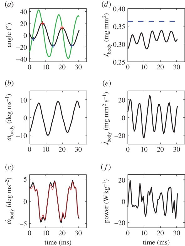
 (black: by differentiation of ωbody; red: according to electronic supplementary material, equation (S3.18)); (d) moment of inertia about the CoM Jbody; dashed blue line shows
  (i.e. Jbody for the straight fish), (e) rate of change of the moment of inertia
  ; (f) total specific body power
  based on the rate of change of kinetic energy.
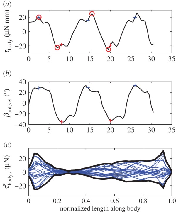
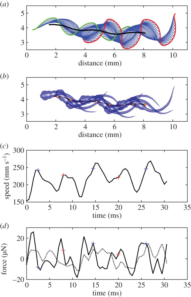
 . Each blue curve represents the torque distribution at a particular instant (at 1 ms intervals). The heavy black curves show the envelope. The narrowest location along of the ‘neck’ of the envelope corresponds to the location of the straight-body CoM.
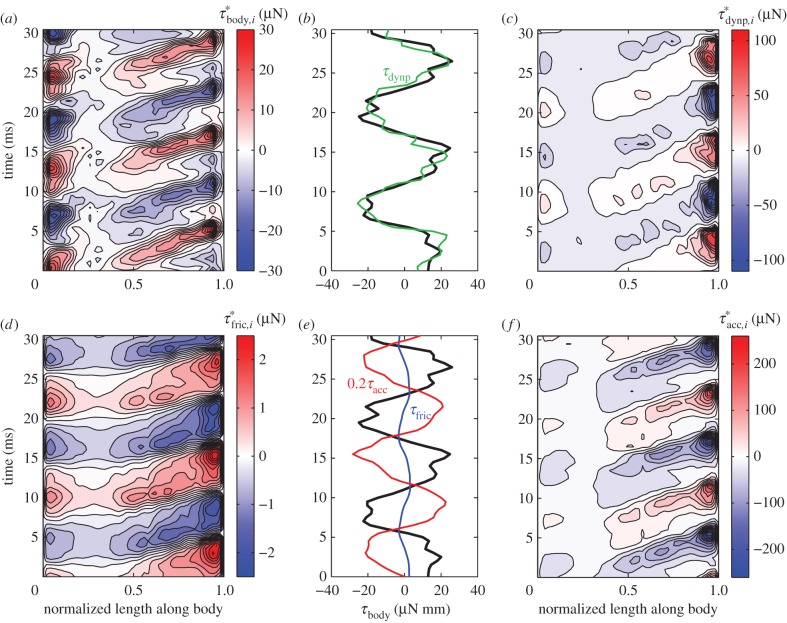
 ) and time. (b) Inertial body torque τbody against time (black); torque on the body due to dynamic pressure, τdynp (green). (c) Contour plot of torque on the body per unit length due to dynamic pressure against
  and time. (d) Contour plot of torque on the body per unit length due to shear-force distribution against
  and time. (e) Inertial body torque τbody against time (black); torque on the body torque due to shear-force distribution, τfric (blue) and acceleration reaction forces (τacc) × 0.2 (red). (f) Contour plot of torque per unit length on the body due to acceleration reaction forces against
  and time.
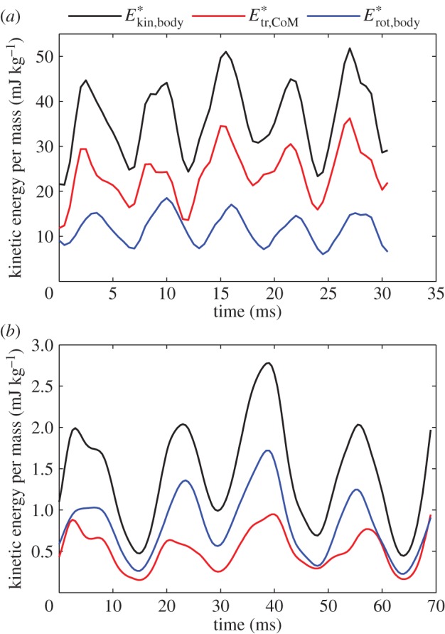
 ; black), kinetic energy due to speed of the CoM (
 ; red), and sum of kinetic energy due to rotation of the segmental masses around CoM and rotation of the segments about their central vertical axis (
 ; blue).
  .
.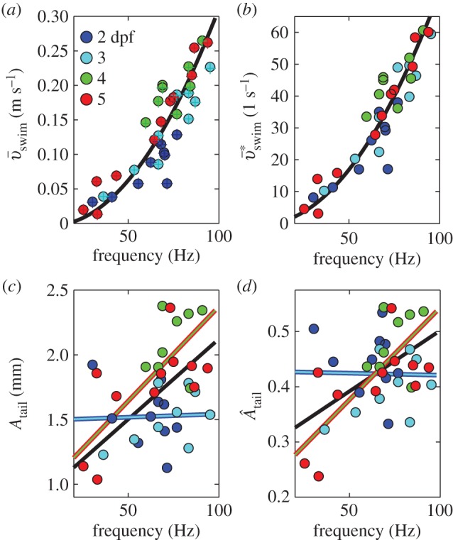
 along the path of the CoM (○) and along a straight line approximation of the path of motion (+) against cycle frequency f. Both speeds differ little, indicating small sideslip. 2, 3 dpf larvae reach lower speeds for a given f than 4, 5 dpf larvae. (b) Specific swimming speed (
 ) against f (same dataset as (a)). (c) Peak-to-peak tail-beat amplitude Atail against f. Data in (c) and (d) were fitted by total least squares. In (c), the black curve shows the fit for the total dataset. The combined datasets for 2 and 3 dpf (blue-cyan line) and 4 and 5 dpf (red-green line) were fitted also separately. The 4–5 dpf age group tended to use higher Atail than the 2–3 dpf group for f > 50 Hz, and they vary Atail more over the frequency range. Panel (d) shows same data as (c) for dimensionless tail-beat amplitude (
 ). Parameter values for each curve fit are given in electronic supplementary material, table S2.
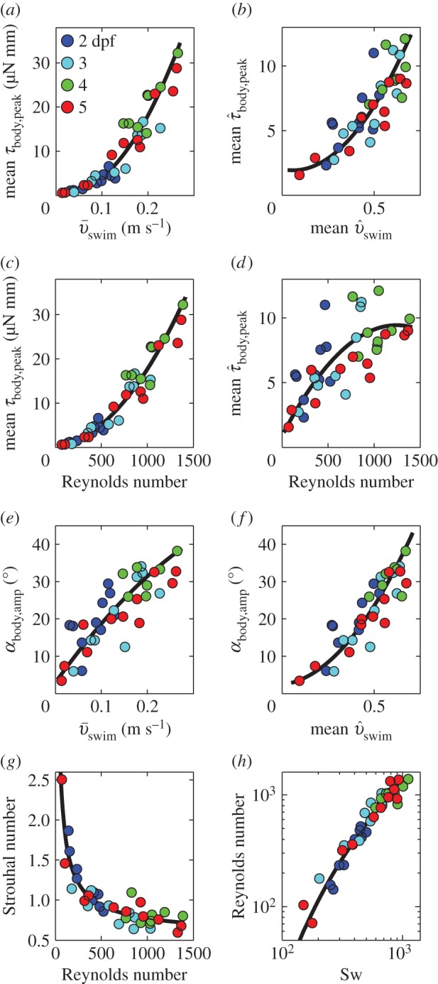
 ). (b) As (a), but non-dimensionalized. (c) Amplitude of torque peaks against Reynolds number (Re). (d) As (c) but non-dimensionalized. (e) Peak-to-peak amplitude of body angle (mean per event) against
  . (f) Idem, but against dimensionless swimming speed. Second-order polynomial curve fits are shown for (a)–(f). (g) St against Re, with a fit of a (negative) power function plus a constant. (h) Re against swimming number Sw (logarithmic scales). The curve fit follows from the fit of St against Re, by using St = Sw/Re. Parameter values for each curve fit are given in electronic supplementary material, table S3.
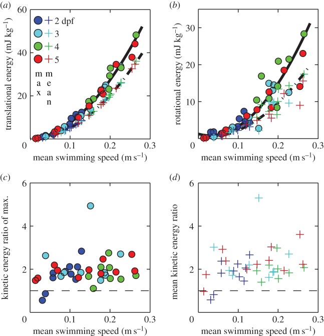
 Second-order polynomial curve fits for maxima (continuous curve) and mean (dashed curve) are shown in (a,b). (c,d) Ratio of the maxima (c) and the means (d) of Etr,CoM and Erot,body over
  . The horizontal dashed line indicates a ratio of 1. Parameter values for each curve fit in (a) and (b) are given in electronic supplementary material, table S4.
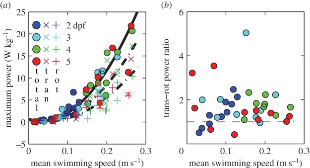
References
-
- Batty RS, Blaxter JHS. 1992. The effect of temperature on the burst swimming performance of fish larvae. J. Exp. Biol. 170, 187–201.
-
- Fuiman LA, Batty RS. 1997. What a drag it is getting cold: partitioning the physical and physiological effects of temperature on fish swimming. J. Exp. Biol. 200, 1745–1755. - PubMed
-
- Osse JWM, van den Boogaart JGM. 1999. Dynamic morphology of fish larvae, structural implications of friction forces in swimming, feeding and ventilation. J. Fish Biol. 55sA, 156–174. (10.1111/j.1095-8649.1999.tb01053.x) - DOI
Publication types
MeSH terms
Associated data
LinkOut - more resources
Full Text Sources
Other Literature Sources
Research Materials
