Visual coding with a population of direction-selective neurons

Abstract

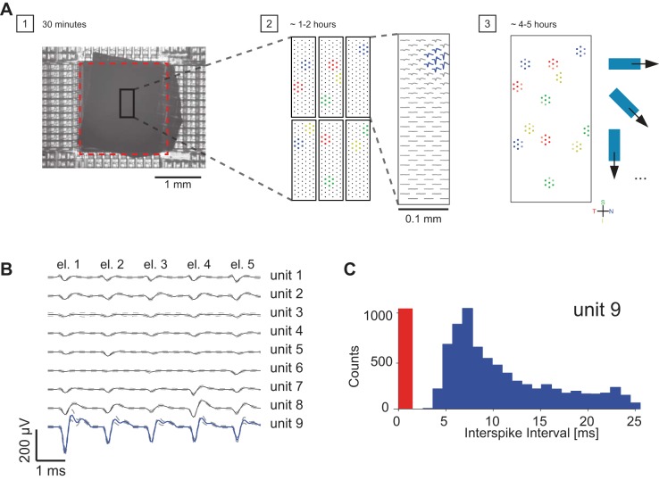
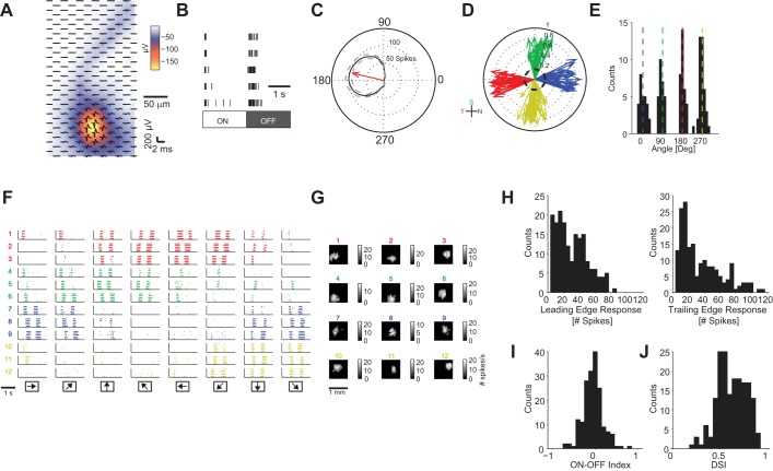
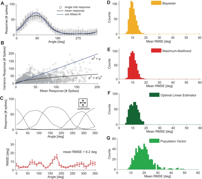
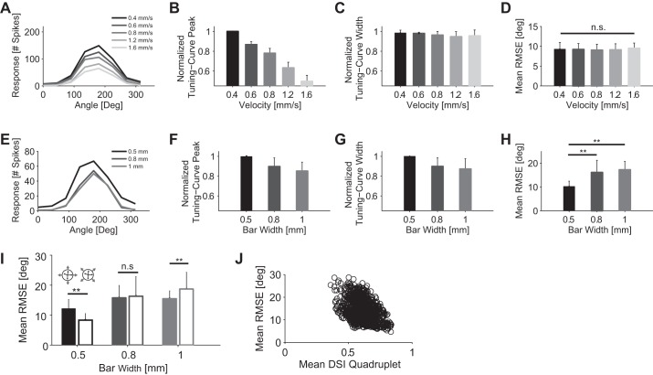
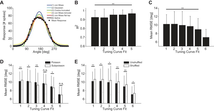
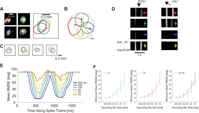
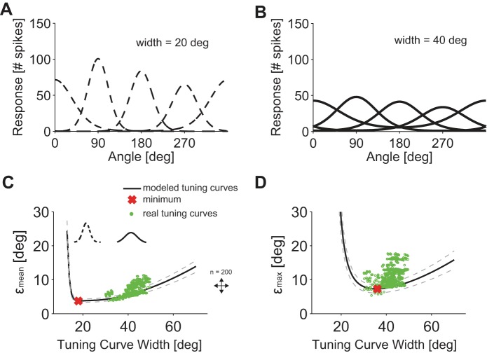
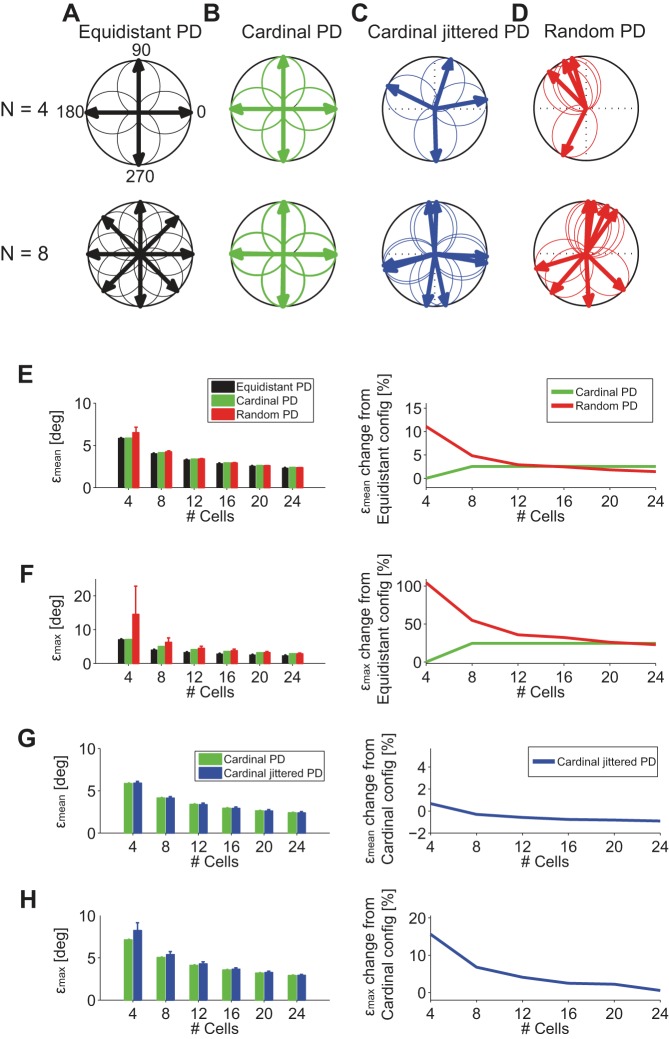
The brain decodes the visual scene from the action potentials of ∼20 retinal ganglion cell types. Among the retinal ganglion cells, direction-selective ganglion cells (DSGCs) encode motion direction. Several studies have focused on the encoding or decoding of motion direction by recording multiunit activity, mainly in the visual cortex. In this study, we simultaneously recorded from all four types of ON-OFF DSGCs of the rabbit retina using a microelectronics-based high-density microelectrode array (HDMEA) and decoded their concerted activity using probabilistic and linear decoders. Furthermore, we investigated how the modification of stimulus parameters (velocity, size, angle of moving object) and the use of different tuning curve fits influenced decoding precision. Finally, we simulated ON-OFF DSGC activity, based on real data, in order to understand how tuning curve widths and the angular distribution of the cells' preferred directions influence decoding performance. We found that probabilistic decoding strategies outperformed, on average, linear methods and that decoding precision was robust to changes in stimulus parameters such as velocity. The removal of noise correlations among cells, by random shuffling trials, caused a drop in decoding precision. Moreover, we found that tuning curves are broad in order to minimize large errors at the expense of a higher average error, and that the retinal direction-selective system would not substantially benefit, on average, from having more than four types of ON-OFF DSGCs or from a perfect alignment of the cells' preferred directions.

Keywords: coding; direction-selective system; microelectrode array; retina; retinal ganglion cells.

Fig. 1.

Method for recording from a defined population of retinal neurons. A: step 1: rabbit retina patch, ganglion cell side down on the electrode array (sensor area is shown by dashed red rectangle). Step 2: scanning of the ganglion cell layer by high-density electrode blocks in order to find locations of defined cell types (indicated by different colors). Step 3: assignment of 5–7 electrodes per ganglion cell for simultaneous recording of light-induced activity from identified and defined populations of retinal neurons. B: average multichannel spike waveforms of 9 spiking units, isolated from 5 neighboring electrodes (el. 1–el. 5) (solid line, mean voltage; dashed line, SD voltage). Electrodes were chosen so as to feature the largest-amplitude signals of the neurons of interest (here, e.g., all 5 electrodes recorded large signals for unit 9). C: interspike interval (ISI) distribution for unit 9 shown in B. The red region indicates the ISI violation time (0–1.5 ms).

Fig. 2.

Extracellular recording from retinal ON-OFF direction-selective ganglion cells (DSGCs). A: spatial profile of an action potential of a single ganglion cell. Red-yellow area, high amplitude signals; black waveform: average single-cell action potential on a single electrode (204 electrodes). Amplitude color scale refers to the minimum of the waveform. B: raster plot of ganglion cell responses to 5 ON and 5 OFF flashing static stimuli. C: tuning curve of ganglion cell responses to motion of a bar. Red arrow points in the preferred direction of the ganglion cell. Black solid line, mean response; dashed gray lines, SD. D: preferred directions of 126 ON-OFF DSGCs recorded from 10 retinas. The length of each vector indicates the magnitude of the direction selectivity index (DSI): 0 = not direction selective, symmetric response; 1 = direction selective, asymmetric response (see materials and methods). T, temporal; S, superior; N, nasal; I, inferior. E: histogram of ON-OFF DSGC vector angles from D. Nasal = 1.4 ± 14.1°, superior = 84.8 ± 10.8°, temporal = 182.8 ± 9.6°, inferior = 268.4 ± 13.1° (mean ± SD). F: raster plot of ganglion cell responses to motion; simultaneous responses of 12 ON-OFF DSGCs. Responses are colored according to the ganglion cell's preferred directions (red, temporal; green, superior; blue, nasal; yellow, inferior). Each row shows the activity of a single ganglion cell for different directions of motion. Arrows at bottom indicate directions of motion. G: receptive field locations of ON-OFF DSGCs in F. H, left: distribution of cell responses for bar leading edge (ON response). Right: distribution of responses for bar trailing edge (OFF response). I: distribution of ON-OFF indexes. J: distribution of DSIs. In H, I, and J, statistics are computed from all 126 recorded ON-OFF DS cells across all stimulus parameters used (see materials and methods).

Fig. 3.

Coding precision of retinal ON-OFF DSGC populations. A: response of a single ON-OFF DSGC to a bar moving along 36 directions, angularly spaced by 10°; n = 100 sweeps per direction. Responses are quantified as the total number of spikes fired by the cell during each stimulus direction (gray circles). The mean response is displayed by the black curve; the von Mises fit to the mean response is displayed by the blue curve. B: characterization of the response variability of ON-OFF DSGCs (n = 126). The response was quantified as the total number of spikes for a given stimulus. The plot displays the correlation between the mean and variance of ON-OFF DSGC responses for all recorded cells and all motion directions across all applied stimulus parameters. Fit: power function: σ_N² = σ_N²(μ) = aμ^b, with a = 4.03 and b = 0.51, where σ² = variance and μ = mean (black line). Poisson variability of responses with a mean equal to the variance is indicated by the blue line. Fano factors of the cells (i.e., the variance of a cell's response to a stimulus divided by its mean) ranged from ∼0.5 (for motion directions close to the preferred direction of the ON-OFF DSGC) to ∼1.5 (for motion directions close to the null direction of the ON-OFF DSGC). C, top: example group of 4 ON-OFF DSGCs used for decoding motion direction (we refer to such a group as a “quadruplet”). Bottom: root mean squared error (RMSE) along 36 different motion directions angularly spaced at 10°. Error bars show SD due to 10-fold cross-validation (see materials and methods). The general decoding performance of this quadruplet can be summarized by a mean RMSE equal to 6.2°. D–G: mean RMSE distributions results for 4 different decoders; each decoder type is indicated in the key [n = 600 quadruplets, bar size = 1 mm × 0.5 mm² (length × width), stimulus velocity = 1.6 mm/s]. Responses were quantified as the total number of spikes fired by the cell during each stimulus.

Fig. 4.

Influence of stimulus velocity and size on decoding performance. A: tuning curves for stimulus velocities ranging from 0.4 to 1.6 mm/s. Bar size was 1 mm × 0.5 mm (length × width). The bar moved along to its long edge. B: normalized tuning curve peak as a function of stimulus velocity. For every cell, each tuning curve peak value, across all stimulus velocities, was normalized with respect to the highest tuning curve peak value (1 indicates highest tuning curve peak; n = 10). C: normalized tuning curve width (computed from von Mises fit) as a function of stimulus velocity. For every cell, each tuning curve width, across all stimulus velocities, was normalized with respect to the highest tuning curve width (1 indicates highest tuning curve width; n = 10). D: mean RMSE for 5 stimulus velocities (n = 108 quadruplets of ON-OFF DSGCs). Decoding performed by von Mises fit, Poisson noise, and a Bayesian decoder. Bar size was 1 × 0.5 mm² (length × width). Responses were quantified as the total number of spikes fired by the cell during each stimulus. E: tuning curves for bar widths ranging from 0.5 to 1 mm. Bar velocity was 1.6 mm/s. F: normalized tuning curve peak as a function of bar width (normalized as in B; n = 10). G: normalized tuning curve width (computed from von Mises fit) as a function of bar size (normalized as in C; n = 10). H: mean RMSE for bars with 3 different widths: 0.5 mm (n = 600 quadruplets of ON-OFF DSGCs), 0.8 mm (n = 159 quadruplets of ON-OFF DSGCs), and 1 mm (n = 464 quadruplets of ON-OFF DSGCs). Decoding performed by von Mises fit, Poisson noise, and a Bayesian decoder. Stimulus velocity was 1.6 mm/s. Responses were quantified as the total number of spikes fired by the cell for each stimulus direction. I: comparison of decoding performance between motion directions close to the cells' preferred directions (filled bars) and motion directions ∼45° away from the cells' preferred directions (open bars). Comparison is reported for 3 different bar widths. Arrow at top indicates the decoded motion directions with respect to the cells' preferred directions. J: correlation plot between DSI and decoding accuracy. x-Axis displays mean DSI of a quadruplet. y-Axis displays mean RMSE obtained from a quadruplet (Pearson correlation coefficient = −0.4). The plot combines the decoding performance of quadruplets across all 3 bar widths (0.5, 0.8, and 1 mm; n = 1223). Error bars indicate SD in all panels. *P < 0.05; **P < 0.01. n.s., Not significant.

Fig. 5.

Influence of tuning curve fit on decoding performance. A: various tuning curve fits. The different fit types are indicated in the key by different colors and numbers. B: mean coefficient of determination R² (10-fold cross-validated) for 126 ON-OFF DSGCs fitted by 5 different functions numbered 1–5 in A. C: average RMSE using 6 different functional fits of the tuning curves. Fits numbered as in A [n = 600 quadruplets, bar size = 0.5 × 1 mm² (length × width), stimulus velocity = 1.6 mm/s]. Decoding results were obtained by using a Bayesian decoder and Poisson noise assumption. Responses were quantified as the total number of spikes fired by the cell for each stimulus. D: comparison of decoding accuracies for Poisson and sub-Poisson noise assumptions across all tuning curve fits [n = 600 quadruplets, bar size = 0.5 × 1 mm² (length × width), stimulus velocity = 1.6 mm/s]. Decoding results were obtained by using a Bayesian decoder, and responses were quantified as the total number of spikes fired by the cell for each stimulus. E: comparison of decoding accuracies between unshuffled and shuffled trials across all tuning curve fits [n = 600 quadruplets, bar size = 0.5 × 1 mm² (length × width), stimulus velocity = 1.6 mm/s]. Decoding results were obtained by using a Bayesian decoder and Poisson noise assumption. Responses were quantified as the total number of spikes fired by the cell for each stimulus. Error bars indicate SD in all panels. *P < 0.05; **P < 0.01.

Fig. 6.

Influence of time bin size on decoding performance. A: overlapping receptive fields of 4 simultaneously recorded ON-OFF DSGCs, fitted by ellipse function. B: tuning curves and preferred directions of the cells in A. C: additional examples of ON-OFF DSGC quadruplets with overlapping receptive fields. D: simultaneous responses of ON-OFF DSGCs in A for a bar moving in the direction indicated by black arrows at top. Each panel shows 100 responses of a single cell. Preferred directions of the respective cells are indicated by colored arrows within the panels. E: decoding performance at consecutive time points of cell responses. Each curve represents decoding results obtained with a different temporal bin size to count cell spikes. For decoding we used a von Mises fit for the tuning curves, Poisson variability of responses, and a Bayesian decoder [bar size = 0.5 × 1 mm² (length × width), stimulus velocity = 1.6 mm/s]. F: decoding performance as a function of bin size (ms) for the 5 quadruplets of ON-OFF DSGCs displayed in A. Decoding performance is reported separately for leading edge (LE; left), trailing edge (TE; center), as well as leading and trailing edges (LE+TE; right).

Fig. 7.

Influence of tuning curve width on decoding precision. A and B: 2 examples (solid and dashed lines, von Mises function) of 4 simulated tuning curves with preferred directions separated by 90° for 2 different widths of 40° and 20°. The integral of the tuning curves was fixed. C: ε_mean, computed with model tuning curves, as a function of the tuning curve width (solid line, mean; dashed line, SD). Red cross, lowest ε_mean value; green dots, ε_mean values for measured tuning curves (n = 600 quadruplets). D: ε_max, computed with model tuning curves, as a function of tuning curve width (solid line, mean; dashed line, SD). Red cross, lowest ε_max value; green dots, ε_max values for measured tuning curves (n = 600, quadruplets).

Fig. 8.

Influence of angular arrangement of and jitter in preferred directions on decoding performance. A, top: 4 direction-selective cells with preferred directions equidistantly spaced by 90°. Bottom: 8 direction-selective cells equidistantly spaced by 45°, “Equidistant PD.” B, top: 4 direction-selective cells with preferred directions equidistantly spaced by 90° and aligned with the 4 cardinal directions. Bottom: 8 direction-selective cells equidistantly spaced by 90° and aligned with the 4 cardinal directions (2 per cardinal direction), “Cardinal PD.” C, top: 4 direction-selective cells with preferred directions jittered around 4 cardinal directions; jitter was obtained from recorded data (Fig. 2E). Bottom: 8 direction-selective cells with preferred directions jittered around 4 cardinal directions, “Cardinal Jittered PD.” D, top: 4 direction-selective cells randomly arranged in the angular space. Bottom: 8 direction-selective cells randomly arranged in the angular space, “Random PD.” E, left: ε_mean as a function of the number of cells and arrangement (Equidistant PD, Cardinal PD, and Random PD) of preferred directions. Right: ε_mean % change with respect to Equidistant PD configuration (n = 200 simulations for every group of cells). F, left: ε_max as a function of the number of cells and arrangement (Equidistant PD, Cardinal PD, and Random PD) of preferred directions. Right: ε_max % change with respect to Equidistant PD configuration. G, left: ε_mean as a function of the number of cells and arrangement (Cardinal PD and Cardinal Jittered PD) of preferred directions. Right: ε_mean % change with respect to “Cardinal PD” configuration. H, left: ε_max as a function of the number of cells and arrangement (Cardinal PD and Cardinal Jittered PD) of preferred directions. Right: ε_max % change with respect to “Cardinal PD” configuration.

References

1. Amthor FR, Grzywacz NM, Merwine DK. Extra-receptive-field motion facilitation in on-off directionally selective ganglion cells of the rabbit retina. Vis Neurosci 13: 303–309, 1996. - PubMed
1. Amthor FR, Oyster CW, Takahashi ES. Morphology of on-off direction-selective ganglion cells in the rabbit retina. Brain Res 298: 187–190, 1984. - PubMed
1. Amthor FR, Takahashi ES, Oyster CW. Morphologies of rabbit retinal ganglion cells with complex receptive fields. J Comp Neurol 280: 97–121, 1989. - PubMed
1. Amthor FR, Tootle JS, Grzywacz NM. Stimulus-dependent correlated firing in directionally selective retinal ganglion cells. Vis Neurosci 22: 769–787, 2005. - PubMed
1. Ariel M, Daw NW. Pharmacological analysis of directionally sensitive rabbit retinal ganglion cells. J Physiol 324: 161–185, 1982. - PMC - PubMed
Publication types
LinkOut - more resources