Physics at the [Formula: see text] linear collider

Abstract

A comprehensive review of physics at an [Formula: see text] linear collider in the energy range of [Formula: see text] GeV-3 TeV is presented in view of recent and expected LHC results, experiments from low-energy as well as astroparticle physics. The report focusses in particular on Higgs-boson, top-quark and electroweak precision physics, but also discusses several models of beyond the standard model physics such as supersymmetry, little Higgs models and extra gauge bosons. The connection to cosmology has been analysed as well.

Fig. 1

The achievable precision in the different Higgs couplings at the LHC on bases of $3a{b}^{-1}$ and 50 % improvement in the theoretical uncertainties in comparison with the different energy stages at the ILC. In the final LC stage all couplings can be obtained in the 1–2 % range, some even better [39]

Fig. 2

Simulated measurement of the background-subtracted $t\overline{t}$ cross section with 10 fb${}^{-1}$ per data point, assuming a top-quark mass of 174 GeV in the 1S scheme with the ILC luminosity spectrum for the CLIC-ILD detector [40]

Fig. 3

Statistical precision on $\mathit{CP}$-conserving form factors expected at the LHC [42] and at the ILC [41]. The LHC results assume an integrated luminosity of $\mathcal{L}=300$ fb${}^{-1}$. The results for the ILC are based on an integrated luminosity of $\mathcal{L}=500$ fb${}^{-1}$ at $\sqrt{s}=500$ GeV and a beam polarisation of $P_{e^{-}}=\pm 80\%$, $P_{e^{+}}=\mp 30\%$ [41]

Fig. 4

Equivalence of the SUSY electroweak Yukawa couplings $g_{\tilde{W}}$, $g_{\tilde{B}}$ with the SU(2), U(1) gauge couplings g, $g^{\prime }$. Shown are the contours of the polarised cross sections ${\mathit{\sigma }}_L(e^{+}{e}^{-}\to {\tilde{\mathit{\chi }}}_1^0{\tilde{\mathit{\chi }}}_2^0)$ and ${\mathit{\sigma }}_R(e^{+}{e}^{-}\to {\tilde{\mathit{\chi }}}_1^0{\tilde{\mathit{\chi }}}_2^0)$ in the plane of the SUSY electroweak Yukawa couplings normalised to the gauge couplings, $Y_L=g_{\tilde{W}}/g$, $Y_R=g_{\tilde{B}}/g^{\prime }$ [43, 44] for a scenario with the electroweak spectrum similar to the reference point SPS1a

Fig. 5

Polarised cross sections versus $P_{e^{-}}$ (bottom panel) and $P_{e^{+}}$ (top panel) for $e^{+}{e}^{-}\to \tilde{e}\tilde{e}$-production with direct decays in ${\tilde{\mathit{\chi }}}_1^{0}e$ in a scenario where the non-coloured spectrum is similar to a SPS1a-modified scenario but with $m_{{\tilde{e}}_L}=200$ GeV, $m_{{\tilde{e}}_R}=195$ GeV. The associated chiral quantum numbers of the scalar SUSY partners ${\tilde{e}}_{L,R}$ can be tested via polarised $e^{\pm }$-beams

Fig. 6

WIMP mass as a function of the mass for p-wave ($J_0=1$) annihilation and under the assumption that WIMP couplings are helicity- and parity-conserving in the process $e^{+}{e}^{-}\to \mathit{\gamma }\mathit{\chi }\mathit{\chi }$ [48]. With an integrated luminosity of $\mathcal{L}=500$ fb${}^{-1}$ and polarised beams with $P_{e^{-}}=+80\%$, $P_{e^{+}}=-60\%$ with $\mathit{\Delta }P/P=0.25\%$ the reconstructed WIMP mass can be determined with a relative accuracy of the order of 1 % [49]. The blue area shows the systematic uncertainty and the red bands the additional statistical contribution. The dominant sources of systematic uncertainties are $\mathit{\Delta }P/P$ and the shape of the beam-energy spectrum

Fig. 7

Combined limits for fermionic dark matter models. The process $e^{+}{e}^{-}\to \mathit{\chi }\mathit{\chi }\mathit{\gamma }$ is assumed to be detected only by the hard photon. The analysis has been modelled correspondingly to [49] and is based on $\mathcal{L}=500$ fb${}^{-1}$ at $\sqrt{s}=500$ GeV and $\sqrt{s}=1$ TeV and different polarisations [50, 51]

Fig. 8

Achievable precision on ${sin}^2{\mathit{\theta }}_{23}$ from bi-linear R-parity-violating decays of the ${\tilde{\mathit{\chi }}}_1^0$ as a function of the produced number of neutralino pairs compared to the current precision from neutrino oscillation measurements [52]

Fig. 9

Theoretical prediction for ${sin}^2{\mathit{\theta }}_{\mathrm{eff}}$ in the SM and the MSSM (including prospective parametric theoretical uncertainties) compared to the experimental precision at the LC with GigaZ option. A SUSY inspired scenario SPS 1a’ has been used, where the coloured SUSY particles masses are fixed to 6 times their SPS 1a’ values. The other mass parameters are varied with a common scale factor

Fig. 10

New gauge bosons in the ${\mathit{\mu }}^{+}{\mathit{\mu }}^{-}$ channel. The plot shows the expected resolution at CLIC with $\sqrt{s}=3$ TeV and $\mathcal{L}=1$ ab${}^{-1}$ on the ‘normalised’ vector $v_f^n=v_f^{\prime }\sqrt{s/(m_Z^{\prime 2}-s)}$ and axial-vector $a_f^n=a_f^{\prime }\sqrt{s/(m_Z^{\prime 2}-s)}$ couplings to a 10 TeV $Z^{\prime }$ in terms of the SM couplings $v_f^{\prime }$, $a_f^{\prime }$. The mass of $Z^{\prime }$ is assumed to be unknown, nevertheless the couplings can be determined up to a two-fold ambiguity. The colours denote different $Z^{\prime }$ models [9, 10]

Fig. 11

Upper plot Event in Higgs-strahlung $e^{+}{e}^{-}\to ZH\to ({\mathit{\mu }}^{+}{\mathit{\mu }}^{-})(\mathrm{jet}\mathrm{jet})$ for a Higgs mass of 125 GeV at a collider energy of 500 GeV; lower plot Distribution of the recoiling Higgs decay jets

Fig. 12

Upper plot Threshold rise of the Cross section for Higgs-strahlung $e^{+}{e}^{-}\to ZH$ corresponding to Higgs spin $=0,1,2$, complemented by the analysis of angular correlations; lower plot Measurements of Higgs couplings as a function of particle masses

Fig. 13

Upper plot reconstructed 2-jet invariant mass for associated production: $e^{+}{e}^{-}\to AH\to b\overline{b}b\overline{b}$ for a Higgs mass of 900 GeV at a collider energy of 3 TeV; lower plot similar plot for $e^{+}{e}^{-}\to H^{+}{H}^{-}\to t\overline{b}\overline{t}b$

Fig. 14

Displays of example Higgs-boson candidate events. Top $H\to ZZ\to 2\mathit{\mu }2e$ candidate in the ATLAS detector; bottom VBF $H\to \mathit{\gamma }\mathit{\gamma }$ candidate in the CMS detector

Fig. 15

Reconstructed distributions of the Higgs boson candidate decay products for the complete 2011/2012 data, expected backgrounds, and simulated signal from top the ATLAS $H\to \mathit{\gamma }\mathit{\gamma }$ [101], centre the CMS $H\to ZZ\to 4\ell$ [102], and bottom the ATLAS $H\to WW\to 2\ell 2\mathit{\nu }$ [103] analyses

Fig. 16

Evidence for the decay $H\to \mathit{\tau }\mathit{\tau }$. Top CMS observed and predicted $m_{\mathit{\tau }\mathit{\tau }}$ distributions [109]. The distributions obtained in each category of each channel are weighted by the ratio between the expected signal and signal-plus-background yields in the category. The inset shows the corresponding difference between the observed data and expected background distributions, together with the signal distribution for a SM Higgs boson at $m_H=125$ GeV; bottom ATLAS event yields as a function of $log(S/B)$, where S (signal yield) and B (background yield) are taken from the corresponding bin in the distribution of the relevant BDT output discriminant [110]

Fig. 17

Higgs boson signal strength as measured by ATLAS for different decay channels [112]

Fig. 18

Higgs-boson production strength, normalised to the SM expectation, based on CMS analyses [113], for a combination of analysis categories related to different production modes.

Fig. 19

Likelihood for the ratio ${\mathit{\mu }}_{\text{VBF}}/{\mathit{\mu }}_{ggF+ttH}$ obtained by ATLAS for the combination of the $H\to \mathit{\gamma }\mathit{\gamma }$, $ZZ\to 4\ell$ and $WW\to 2\mathit{\nu }2\ell$ channels and $m_H=125.5$ GeV [112]

Fig. 20

Preliminary ATLAS results of fits for a two-parameter benchmark model that probes different coupling strength scale factors common for fermions (${\mathit{\kappa }}_F$) and vector bosons (${\mathit{\kappa }}_V$), respectively, assuming only SM contributions to the total width. Shown are 68 and 95 % CL contours of the two-dimensional fit; overlaying the 68 % CL contours derived from the individual channels and their combination. The best-fit result ($\times$) and the SM expectation ($+$) are also indicated [112]

Fig. 21

Test of custodial symmetry: CMS likelihood scan of the ratio ${\mathit{\lambda }}_{WZ}$, where SM coupling of the Higgs bosons to fermions are assumed [113]

Fig. 22

Constraining BSM contributions to particle loops: CMS 2d likelihood scan of gluon and photon coupling modifiers ${\mathit{\kappa }}_g$, ${\mathit{\kappa }}_{\mathit{\gamma }}$ [113]

Fig. 23

Summary plot of CMS likelihood scan results [113] for the different parameters of interest in benchmark models documented in [38]. The inner bars represent the 68 % CL confidence intervals, while the outer bars represent the 95 % CL confidence intervals

Fig. 24

ATLAS summary of the fits for modifications of the SM Higgs-boson couplings expressed as a function of the particle mass. For the fermions, the values of the fitted Yukawa couplings for the $Hf\overline{f}$ vertex are shown, while for vector bosons the square-root of the coupling for the HVV vertex divided by twice the vacuum expectation value of the Higgs boson field [112]

Fig. 25

CMS mass measurements [113] in the $\mathit{\gamma }\mathit{\gamma }$ and $ZZ\to 4\ell$ final states and their combinations. The vertical band shows the combined uncertainty. The horizontal bars indicate the $\pm 1$ standard deviation uncertainties for the individual channels

Fig. 26

Observed transverse mass distributions for the ATLAS $ZZ\to 2\ell 2\mathit{\nu }$ analysis [115] in the signal region compared to the expected contributions from ggF and VBF Higgs production with the decay $H^{\ast }\to ZZ$ SM and with ${\mathit{\mu }}_{\text{off-shell}}=10$ (dashed) in the $2e2\mathit{\nu }$ channel. A relative $gg\to ZZ$ background K-factor of 1 is assumed

Fig. 27

CMS likelihood scan versus ${\mathit{\Gamma }}_H$. Different colours refer to: combination of $4\ell$ low-mass and high-mass (ochre), combination of $4\ell$ low-mass and $2\ell 2\mathit{\nu }$ high-mass and combination of $4\ell$ low-mass and both channels at high-mass (blue). Solid and dashed lines represent observed and expected limits, respectively [116]

Fig. 28

Top final-state observables sensitive to the spin and parity of the decaying resonance in $Z{Z}^{\ast }\to 4\ell$ final states. Bottom $cos{\mathit{\theta }}_1$ distribution for ATLAS data (point with errors), the backgrounds (filled histograms) and several spin hypotheses (SM solid line and alternatives dashed lines) [119]

Fig. 29

Distributions of the test statistic $q=-2ln({\mathcal{L}}_{J^P}/{\mathcal{L}}_{0^{+}})$ for the spin-1 and spin-2 JP models tested against the SM Higgs boson hypothesis in the combined $X\to ZZ$ and WW analyses [117]. The expected median and the 68.3, 95.4, and 99.7 % CL regions for the SM Higgs boson (orange, the left for each model) and for the alternative $J^P$ hypotheses (blue, right) are shown. The observed q values are indicated by the black dots

Fig. 30

Projected a diphoton mass distribution for the SM Higgs boson signal and background processes after VBF selection and b background-subtracted dimuon mass distribution based on ATLAS simulations assuming an integrated luminosity of 3000 fb${}^{-1}$ [138]

Fig. 31

Relative uncertainty on the signal strength determination expected for the ATLAS experiment [136]. Assuming a SM Higgs boson with a mass of 125 GeV and 300 fb${}^{-1}$ and 3000 fb${}^{-1}$ of 14 TeV data. The uncertainty pertains to the number of events passing the experimental selection, not to the particular Higgs boson process targeted. The hashed areas indicate the increase of the estimated error due to current theory systematic uncertainties

Fig. 32

Expected ATLAS 68 and 95 % CL likelihood contours for ${\mathit{\kappa }}_V$ and ${\mathit{\kappa }}_F$ in a minimal coupling fit for an integrated luminosity of 300 fb${}^{-1}$ and 3000 fb${}^{-1}$ [136]

Fig. 33

CMS projected relative uncertainty on the measurements of ${\mathit{\kappa }}_{\mathit{\gamma }}$, ${\mathit{\kappa }}_V$, ${\mathit{\kappa }}_g$, ${\mathit{\kappa }}_b$, ${\mathit{\kappa }}_t$, and ${\mathit{\kappa }}_{\mathit{\tau }}$ assuming $\sqrt{s}=14$ TeV and an integrated luminosity 300 and 3000 fb${}^{-1}$. The results are shown for two uncertainty scenarios described in the text [137]

Fig. 34

Relative uncertainty expected for the ATLAS experiment on the determination of coupling scale factor ratios ${\mathit{\lambda }}_{XY}={\mathit{\kappa }}_X/{\mathit{\kappa }}_Y$ from a generic fit [136], assuming a SM Higgs boson with a mass of 125 GeV and 300 fb${}^{-1}$ and 3000 fb${}^{-1}$ of 14 TeV data. The hashed areas indicate the increase of the estimated error due to current theory uncertainties

Fig. 35

Fit results for the reduced coupling scale factors for weak bosons and fermions as a function of the particle mass, assuming 300/fb or 3000/fb of 14 TeV data and a SM Higgs boson with a mass of 125 GeV [136]

Fig. 36

Projected diphoton mass distribution for signal and background processes based on ATLAS simulations for a search for Higgs boson pair production with subsequent decays $H\to b\overline{b}$ and $H\to \mathit{\gamma }\mathit{\gamma }$ assuming an integrated luminosity of 3000 fb${}^{-1}$ [139]. The simulated distributions are scaled to match the expected event yields but do not necessarily reflect the corresponding statistical fluctuations

Fig. 37

The origin of XVV coupling and its relation to the mass term of V

Fig. 38

$X\to Z{Z}^{\ast }$ decay and $e^{+}{e}^{-}\to ZX$ process

Fig. 39

Mass–coupling relation [144]

Fig. 40

Two proposed detector concepts for the ILC: ILD (left) and SiD (right) [147]

Fig. 41

Why 250–500 GeV? The three thresholds

Fig. 42

Cross sections for the three major Higgs production processes as a function of centre-of-mass energy

Fig. 43

Recoil mass distribution for the process: $e^{+}{e}^{-}\to Zh$ followed by $Z\to {\mathit{\mu }}^{+}{\mathit{\mu }}^{-}$ decay for $m_h=125$ GeV with 250 fb${}^{-1}$ at $\sqrt{s}=250$ GeV [151]

Fig. 44

Threshold scan of the $e^{+}{e}^{-}\to Zh$ process for $m_h=120$ GeV, compared with theoretical predictions for $J^P=0^{+}$, $1^{-}$, and $2^{+}$ [156]

Fig. 45

Determination of $\mathit{CP}$ mixing with $1\mathit{\sigma }$ bands expected at $\sqrt{s}=350$ GeV and 500 fb${}^{-1}$ [158]

Fig. 46

Cross sections for the signal $t\overline{t}h$ process with and without the non-relativistic QCD (NRQCD) correction together with those for the background processes: $t\overline{t}Z,t\overline{t}g(g\to b\overline{b})$ and $t\overline{t}$ (upper plot). The invariant mass distribution for the $t\overline{t}$ subsystem with and without the NRQCD correction (lower plot)

Fig. 47

Cross sections for the double Higgs production processes, $e^{+}{e}^{-}\to Zhh$ and $e^{+}{e}^{-}\to \mathit{\nu }\overline{\mathit{\nu }}hh$, as a function of $\sqrt{s}$ for $m_h=120$ GeV

Fig. 48

Diagrams contributing to a $e^{+}{e}^{-}\to Zhh$ and b $e^{+}{e}^{-}\to \mathit{\nu }\overline{\mathit{\nu }}hh$

Fig. 49

(Upper plot) cross section for $e^{+}{e}^{-}\to Zhh$ at $\sqrt{s}=500$ GeV normalised by that of the SM as a function of the self-coupling normalised by that of the SM. (Lower plot) a similar plot for $e^{+}{e}^{-}\to \mathit{\nu }\overline{\mathit{\nu }}hh$ at $\sqrt{s}=1$ TeV

Fig. 50

Expected mass–coupling relation for the SM case after the full ILC programme

Fig. 51

Comparison of the capabilities of the LHC and the ILC, when the ILC data in various stages: ILC1 with 250 fb${}^{-1}$ at $\sqrt{s}=250$, ILC: 500 fb${}^{-1}$ at 500 GeV, and ILCTeV: $1a{b}^{-1}$ at 1 TeV are cumulatively added to the LHC data with 300 fb${}^{-1}$ at 14 TeV [197]

Fig. 52

Comparison of the model-discrimination capabilities of the LHC and the ILC [200]

Fig. 53

Comparison of the model-discrimination capabilities of the LHC and the ILC [200]

Fig. 54

Comparison of the model-discrimination capabilities of the LHC and the ILC [200]

Fig. 55

Possible machine upgrade scenarios for the ILC [141, 201]

Fig. 56

Longitudinal cross section of the top quadrant of CLIC_SiD (left) and CLIC_ILD (right) [9, 10]

Fig. 57

Reconstructed particles in a simulated $e^{+}{e}^{-}\to H^{+}{H}^{-}\to t\overline{b}\overline{t}b$ event at $\sqrt{s}$=3 TeV in the CLIC_ILD detector including the background from $\mathit{\gamma }\mathit{\gamma }\to \text{hadrons}$ before (left) and after (right) applying tight timing cuts on the reconstructed cluster times [9, 10]

Fig. 58

Search reach in the $m_{\mathrm{A}}-tan\mathit{\beta }$ plane for LHC and CLIC. The left-most coloured regions are current limits from the Tevatron with $\sim$7.5 ${\mathrm{fb}}^{-1}$ of data at $\sqrt{s}=1.96$ TeV and from $\sim$1 ${\mathrm{fb}}^{-1}$ of LHC data at $\sqrt{s}=7$ TeV. The black line is projection of search reach at LHC with $\sqrt{s}=14$ TeV and 300 ${\mathrm{fb}}^{-1}$ of luminosity [211]. The right-most red line is search reach of CLIC in the HA mode with $\sqrt{s}=3$ TeV. This search capacity extends well beyond the LHC [9, 10]

Fig. 59

Di-jet invariant mass distributions for the $e^{+}{e}^{-}\to HA\to b\overline{b}b\overline{b}$ (left) and the $e^{+}{e}^{-}\to H^{+}{H}^{-}\to t\overline{b}\overline{t}b$ (right) signal together with the individual background contributions for model I [9, 10].

Fig. 60

Di-jet invariant mass distributions for the $e^{+}{e}^{-}\to HA\to b\overline{b}b\overline{b}$ (left) and the $e^{+}{e}^{-}\to H^{+}{H}^{-}\to t\overline{b}\overline{t}b$ (right) signal together with the individual background contributions for model II [9, 10]

Fig. 61

$M_A$–$tan\mathit{\beta }$ plane in the $m_h^{max}$ scenario (upper) and in the $m_h^{\mathrm{mod}+}$ scenario (lower plot) [238]. The green-shaded area yields $M_h\sim 125\pm 3\mathrm{GeV}$, the red area at high $tan\mathit{\beta }$ is excluded by LHC heavy MSSM Higgs-boson searches, the blue area is excluded by LEP Higgs searches, and the red strip at low $tan\mathit{\beta }$ is excluded by the LHC SM Higgs searches

Fig. 62

Fit for the light $\mathcal{CP}$-even Higgs mass in the CMSSM (left) and NUHM1 (right) [254]. Direct searches for the light Higgs boson are not included

Fig. 63

Stop mixing parameter $X_t/m_{{\tilde{q}}_3}$ vs. the light stop mass (left), and the light vs. heavy stop masses (right), see text

Fig. 64

The decay branching ratios of H, A and $H^{\pm }$ in 2HDMs for Type I, Type II, Type X and Type Y as a function of $tan\mathit{\beta }$ with $m_H=m_A=m_{H^{\pm }}=250$ GeV and $sin(\mathit{\beta }-\mathit{\alpha })=1$ [295]

Fig. 65

The constraint on the parameter space in the 2HDM for Type I, Type II, Type IV (Type X) and Type III (Type Y) from various flavour experiments [311]

Fig. 66

Expected exclusion regions ($2\mathit{\sigma }$ CL) in the plane of $tan\mathit{\beta }$ and the mass scale $m_{\mathit{\varphi }}$ of the additional Higgs bosons at the LHC. Curves are evaluated by using the signal and background analysis given in Ref. [338] for each process, where the signal events are rescaled to the prediction in each case [339, 340], except the $4\mathit{\tau }$ process for which we follow the analysis in Ref. [341]. Thick solid lines are the expected exclusion contours by $L=300$ fb${}^{-1}$ data, and thin dashed lines are for $L=3000$ fb${}^{-1}$ data. For Type-II, the regions indicated by circles may not be excluded by $H/A\to {\mathit{\tau }}^{+}{\mathit{\tau }}^{-}$ search by using the 300 fb${}^{-1}$ data due to the large SM background

Fig. 67

Contour plots of the four-particle production cross sections through the H / A production and $H^{\pm }$ production process at the ILC with $\sqrt{s}=500$  GeV in the $(m_{H^{\pm }},tan\mathit{\beta })$ plane. Contour of $\mathit{\sigma }=0.1$ fb is drawn for each signature [295]

Fig. 68

Contour plots of the four-particle production cross sections through the H / A production and $H^{\pm }$ production process at the ILC with $\sqrt{s}=1$  TeV in the $(m_{H^{\pm }},tan\mathit{\beta })$ plane. Contour of $\mathit{\sigma }=0.1$ fb is drawn for each signature [295]

Fig. 69

Left the scaling factors in 2HDM with four types of Yukawa interactions. Right the scaling factors in models with universal Yukawa couplings. The current LHC bounds and the expected LHC and ILC sensitivities are also shown at the 68.27 % CL. For details, see Refs. [339, 340]

Fig. 70

Predictions of various scale factors on the ${\mathit{\kappa }}_{\mathit{\tau }}$ vs. ${\mathit{\kappa }}_b$ (upper panel), and ${\mathit{\kappa }}_{\mathit{\tau }}$ vs ${\mathit{\kappa }}_c$ (bottom panel) in four types of Yukawa interactions in the cases with $cos(\mathit{\beta }-\mathit{\alpha })<0$ [293, 294]. Each black dot shows the tree-level result with $tan\mathit{\beta }$=1, 2, 3 and 4. One-loop corrected results are indicated by red for ${sin}^2(\mathit{\beta }-\mathit{\alpha })=0.99$ and blue for ${sin}^2(\mathit{\beta }-\mathit{\alpha })=0.95$ regions where $m_{\mathrm{\Phi }}$ and M are scanned over from 100 GeV to 1 TeV and 0 to $m_{\mathrm{\Phi }}$, respectively. All the plots are allowed by the unitarity and vacuum stability bounds

Fig. 71

Contour plots of the deviation in the hhh coupling in the $(m_{\mathrm{\Phi }}^{},M)$ plane for $m_h=125$ GeV and $sin(\mathit{\beta }-\mathit{\alpha })=1$. The red line indicates ${\mathit{\phi }}_c/T_c=1$, above which the strong first order phase transition occurs (${\mathit{\phi }}_c/T_c>1$) [363, 364]

Fig. 72

Constraints from the unitarity and vacuum stability bounds for ${\mathit{\lambda }}_1=m_h^2/(2v^2)\simeq 0.13$ in the ${\mathit{\lambda }}_4$–${\mathit{\lambda }}_5$ plane. We take ${\mathit{\lambda }}_{\mathit{\Delta }}=1.5$ for the left panel and ${\mathit{\lambda }}_{\mathit{\Delta }}=3$ for the right panel with ${\mathit{\lambda }}_{\mathit{\Delta }}={\mathit{\lambda }}_2={\mathit{\lambda }}_3$ [375]

Fig. 73

Decay branching ratio of $H^{++}$ as a function of $v_{\mathit{\Delta }}$. In the left figure, $m_{H^{++}}$ is fixed to be 300 GeV, and $\mathit{\Delta }m$ is taken to be zero. In the middle figure, $m_{H^{++}}$ is fixed to be 320 GeV, and $\mathit{\Delta }m$ is taken to be 10 GeV. In the right figure, $m_{H^{++}}$ is fixed to be 360 GeV, and $\mathit{\Delta }m$ is taken to be 30 GeV

Fig. 74

Decay branching ratio of $H^{++}$ as a function of $v_{\mathit{\Delta }}$ with $m_{H^{+}}=m_{H^{++}}$. The solid, dashed and dotted curves, respectively, show the results in the case of $m_{H^{++}}=150$, 300 and 500 GeV [375]

Fig. 75

The signal cross section as a function of $m_{H^{++}}$ with the collision energy to be 7 TeV from Ref. [399]. The light (dark) shaded band shows the 95 % CL (expected) upper bound for the cross section from the data with the integrate luminosity to be 4.7 fb${}^{-1}$ (20 fb${}^{-1}$)

Fig. 76

Production cross section of the $e^{+}{e}^{-}\to H^{++}{H}^{--}$ process as a function of $m_{H^{++}}$. The black, blue and red curves are, respectively, the results with the collision energy $\sqrt{s}=$250, 500 and 1000 GeV

Fig. 77

The invariant mass distribution (left panel) and the transverse mass distribution (right panel) for the ${\ell }^{+}{\ell }^{+}$ and ${\ell }^{+}{\ell }^{+}{E}_{\text{miss}}$ systems, respectively, in the case of $m_{H^{++}}=230$ GeV and $\sqrt{s}=500$ GeV [375]. The integrated luminosity is assumed to be 500 fb${}^{-1}$

Fig. 78

The scaling factors in models with universal Yukawa couplings. The current LHC bounds and the expected LHC and ILC sensitivities are also shown at the 68.27 % CL. For details, see Ref. [340]

Fig. 79

Higgs boson branching ratios in MCHM5 as a function of $\mathit{\xi }$ for $M_h=125$ GeV

Fig. 80

Generic Feynman diagrams contributing to Higgs pair production via Higgs-strahlung off Z bosons

Fig. 81

Generic Feynman diagrams contributing to Higgs pair production via W boson fusion

Fig. 82

The ZHH (upper two) and WW fusion (lower two) cross sections in the SM (red) and the MCHM5 for $\mathit{\xi }=0.2$ (blue), $\mathit{\xi }=0.5$ (black) and $\mathit{\xi }=0.8$ (green) divided by the cross section of the corresponding model at $\mathit{\kappa }$=1, as a function of $\mathit{\kappa }$, for $\sqrt{s}=500$ GeV and $\sqrt{s}=1$ TeV

Fig. 83

Summary plot of the current constraints and prospects for direct and indirect probes of Higgs compositeness. The dark brown region shows the current LHC limit from direct search for vector resonance. The dark (medium light) horizontal purple bands indicate the sensitivity on $\mathit{\xi }$ expected at the LHC from double (single) Higgs production with 300 fb${}^{-1}$ of integrated luminosity. The pink horizontal band reports the sensitivity reach on $\mathit{\xi }$ from the study of double Higgs processes alone at CLIC with $1a{b}^{-1}$ of integrated luminosity at 3 TeV, while the light-blue horizontal band shows the sensitivity reach on $\mathit{\xi }$ when considering single Higgs processes. Finally, experimental electroweak precision tests (EWPT) favour the region below the orange thick line with and without additional contributions to $\mathit{\Delta }\mathit{\rho }$. From Ref. [441]

Fig. 84

Scan over the Higgs-portal potential Eq. 68. We include the constraints from electroweak precision measurements

Fig. 85

95% confidence level contours for a measurement of ${\mathit{\Gamma }}_1^{\text{hid}}/{\mathit{\Gamma }}_1^{\text{SM}}$ at the LHC and a $350\text{GeV}$ LC. We use Sfitter [459] for the LHC results and we adopt the linear collider uncertainties of reference [458]

Fig. 86

Measurement of a hypothetical portal model at a 350 GeV linear collider, uncertainties are adopted from Ref. [458]. A measurement of ${\mathcal{R}}_2$ at the LHC, with only an upper 95 % confidence level bound on ${\mathcal{J}}_2$ does not constrain the region ${\mathit{\Gamma }}_2^{\text{hid}}/{\mathit{\Gamma }}_{\text{tot},2}^{\text{SM}}$ below the ${\mathcal{J}}_2$ curve. This degeneracy is lifted with a measurement at a linear collider

Fig. 87

The reduced signal cross section $R_1^{bb}$ at a $e^{+}{e}^{-}$ collider as defined in the text, as a function of $M_{H_1}$ in the semiconstrained NMSSM (from [482])

Fig. 88

The reduced signal cross section $R_2^{bb}$ as function of $M_{H_1}$ in the semiconstrained NMSSM (from [482]).

Fig. 89

Higgs production cross sections at a $e^{+}{e}^{-}$ collider in the channels $Z{H}_1$, $Z{H}_2$, $H^{+}{H}^{-}$ and $H_i{A}_j$ for a point in the parameter space of the semiconstrained NMSSM with Higgs masses as indicated in the text, from [492]

Fig. 90

The reduced coupling $R^{\mathit{\gamma }\mathit{\gamma }}$, as defined in Eq. (81), as function of $M_{{\mathrm{chargino}}_1}$ for $M_{A_S}\sim M_{H_S}\sim 260$ GeV, for a scenario explaining a 130 GeV photon line from dark matter annihilation in the galactic centre

Fig. 91

The reduced coupling $R^{\mathit{\gamma }\mathit{\gamma }}$ as a function of $M_{A_S}$, for points in the semiconstrained NMSSM where $H_S$ with $M_{H_S}\sim 100$ GeV explains the excess in bb at LEP II (from [492]; orange diamonds satisfy the WMAP constraint on the dark matter relic density)

Fig. 92

The reduced coupling $R^{\mathit{\gamma }\mathit{\gamma }}$ as a function of $M_{H_S}$, for points in the semiconstrained NMSSM where $H_S$ with $M_{H_S}\sim 100$ GeV explains the excess in bb at LEP II (from [492]; orange diamonds satisfy the WMAP constraint on the dark matter relic density)

Fig. 93

Accessible range of $\mathit{\Gamma }(h\to gg)$ and $\mathit{\Gamma }(h\to \mathit{\gamma }\mathit{\gamma })$ normalised to the SM value in the LLH model (from [524])

Fig. 94

The $\mathit{\Gamma }(h\to gg)$ normalised to the SM value (from [528]). The $f_{\min }$ is defined as the smallest value allowed by electroweak precision measurements and the values are 1.2 TeV for the LLH model, 500 GeV for T-parity case, 700 GeV for custodial littlest Higgs model and 500 GeV for minimal composite Higgs model, respectively (for details, see [528])

Fig. 95

The (a) shows the total decay width normalised to the SM value in the LHT (from [526]). The difference between case A and case B comes from the definition of the down-type Yukawa term (for details, see [526]). The (b) shows the partial Higgs branching ratios normalised to the SM value (from [526])

Fig. 96

The distribution of $\mathit{\gamma }\mathit{\gamma }$ and $e\mathit{\gamma }$ centre-of-mass energy W with respect to the $e^{+}{e}^{-}$ energy (2$E_0$) from simulation of the PLC luminosity spectra [603]. Contributions of various spin states of produced system are shown

Fig. 97

Distributions of the corrected invariant mass, $W_{\mathrm{corr}}$, for selected $b\overline{b}$ events; contributions of the signal, for $M_{H_{\mathrm{SM}}}=$ 120 GeV, and of the different background processes, are shown separately [613]

Fig. 98

Ratio ${\displaystyle \frac{\mathit{\Gamma }(h\to \mathit{\gamma }\mathit{\gamma })}{\mathit{\Gamma }{(h\to \mathit{\gamma }\mathit{\gamma })}^{\mathrm{SM}}}}$ as a function of the mass scale of the new physics f in the Littlest Higgs model [524], for different Higgs-boson masses. “Accessible” indicates the possible variation of the rate for fixed f labelfig

Fig. 99

Top production of A and H, with parameters corresponding to the LHC wedge, at the $\mathit{\gamma }\mathit{\gamma }$ collider. Exclusion and discovery limits obtained for NLC collider for $\sqrt{ee}=$630 GeV, after 2 or 3 years of operation [642], Bottom the case $M_H=M_A=300$ GeV at ${\mathit{\chi }}_V^H\approx 0$ in the MSSM. Distributions of the corrected invariant mass $W_{corr}$ for selected $b\overline{b}$ events at $tan\mathit{\beta }=7$ [643]

Fig. 100

The specific decay angular distributions ${\mathrm{\Sigma }}_i$ in the $\mathit{\gamma }\mathit{\gamma }\to h^{(i)}\to t\overline{t}$ process in dependence on the $t\overline{t}$ invariant mass for the scalar (dashed) and pseudoscalar (thick solid) $h^{(i)}$ with $M_H=400$ GeV [649]

Fig. 101

The top quark production cross section R for $m_t=170\mathrm{GeV}$ and three values for top quark width. The LO formula for the cross section and ${\mathit{\alpha }}_s(30\mathrm{GeV})=0.142$ is used

Fig. 102

Total cross section for top quark production near threshold at NNNLO (with an estimated third order matching coefficients) and NNLO from [761], where a scale variation of $(20-80)\mathrm{GeV}$ is shown by the coloured bands. A top quark PS mass $m_{\mathrm{PS}}(20\mathrm{GeV})=175\mathrm{GeV}$ is used

Fig. 103

The threshold cross section at fixed order (upper pannel) and renormalisation group improvement (lower pannel) is shown from Ref. [756]. The bands between two coloured lines at each orders show the scale dependence of the results. The RG improved cross sections are stable against scale variation, while fixed order result suffers from large dependence on values of ${\mathit{\mu }}_s$

Fig. 104

Corrections due to Higgs exchange in $e^{+}{e}^{-}\to t\overline{t}$. In the left diagram the Higgs exchange contributes to the production vertex for $\mathit{\gamma }t\overline{t},Zt\overline{t}$, which occurs at short distance when the $t\overline{t}$-pair is separated by $r\sim 1/m_t$. In the right diagram Higgs exchanges occurs after bound-state formation between top and anti-top quarks separated by the scale of the bound state $r\sim 1/(m_t{\mathit{\alpha }}_s)$

Fig. 105

Cross section for $e^{+}{e}^{-}\to t\overline{t}$ for $m_t=170\mathrm{GeV}$ with/without one-loop Higgs boson corrections. A Higgs-boson mass of $m_h=125\mathrm{GeV}$ is used

Fig. 106

Top quark momentum distribution at $\mathit{\Delta }E=E-E_1=0,2,5$ GeV (top) for $m_t=170$ GeV and top-quark mass dependence (bottom) on the momentum distribution

Fig. 107

Dependence of the forward–backward asymmetry $A_{\mathrm{FB}}$ on the top quark width (upper plot) and the strong coupling ${\mathit{\alpha }}_s$ (lower plot). Figures are taken from Ref. [779]

Fig. 108

The top-quark production cross section calculated with TOPPIK for a top mass of 174 GeV in the 1S mass scheme, showing the effects of initial-state radiation and of the luminosity spectrum of CLIC. Figure taken from Ref. [40]

Fig. 109

Simulated measurement of the background-subtracted $t\overline{t}$ cross section with 10 fb${}^{-1}$ per data point, assuming a top-quark mass of 174 GeV in the 1S scheme with the ILC luminosity spectrum for the CLIC_ILD detector. Figure taken from Ref. [40]

Fig. 110

Simulated measurement of the top-quark invariant mass in the all-hadronic decay channel of top-quark pairs for an integrated luminosity of 100 fb${}^{-1}$ at CLIC in the CLIC_ILD detector at a centre-of-mass energy of 500 GeV. The solid green histogram shows the remaining non $t\overline{t}$ background in the data sample. The mass is determined with an unbinned maximum likelihood fit to the distribution. Figure taken from Ref. [40]

Fig. 111

Statistical precision on $M_W$ from the Voigtian fit (see text)

Fig. 112

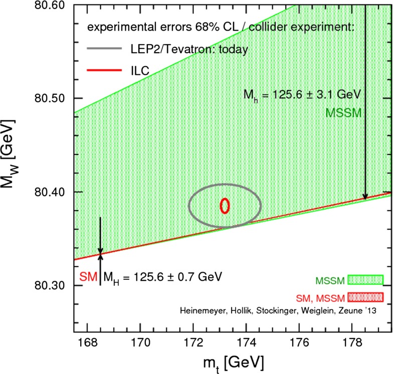
Prediction for $M_W$ as a function of $m_t$. The plot shows the $M_W$ prediction assuming the light $\mathcal{CP}$-even Higgs h in the region $125.6\pm 3.1\mathrm{GeV}$. The red band indicates the overlap region of the SM and the MSSM with $M_H^{\mathrm{SM}}=125.6\pm 3.1$ GeV. All points are allowed by HiggsBounds. The grey ellipse indicates the current experimental uncertainty, whereas the red ellipse shows the anticipated future ILC/GigaZ precision

Fig. 113

Theoretical prediction for ${sin}^2{{\mathit{\theta }}^{\ell }}_{\mathrm{eff}}$ in the SM and the MSSM (including prospective parametric theoretical uncertainties) compared to the experimental precision at the LC with GigaZ option. An SPS 1a${}^{\prime }$ inspired scenario is used, where the squark and gluino mass parameters are fixed to 6 times their SPS 1a${}^{\prime }$ values. The other mass parameters are varied with a common scale factor

Fig. 114

MSSM parameter scan for $M_W$ and ${sin}^2{{\mathit{\theta }}^{\ell }}_{\mathrm{eff}}$ over the ranges given in Eq. (116) with $m_t=165\dots 175\mathrm{GeV}$. Todays 68 % CL ellipses (from $A_{\mathrm{FB}}^b(\mathrm{LEP})$, $A_{\mathrm{LR}}^e(\mathrm{SLD})$ and the world average) are shown as well as the anticipated GigaZ/MegaW precisions, drawn around todays central value

Fig. 115

Loop contribution of the top quark to the Higgs-boson mass

Fig. 116

$\mathit{\Delta }{\mathit{\chi }}^2$ profiles as a function of the Higgs mass for electroweak fits compatible with an SM Higgs boson of mass 125.8 $\mathrm{GeV}$ (left) and 94 $\mathrm{GeV}$ (right), respectively. The measured Higgs-boson mass is not used as input in the fit. The grey bands show the results obtained using present uncertainties [890], and the yellow bands indicate the results for the hypothetical future scenario given in Table 28 (left plot) and corresponding input data shifted to accommodate a 94 $\mathrm{GeV}$ Higgs boson but unchanged uncertainties (right plot). The right axes depict the corresponding Gaussian ‘sigma’ lines. The thickness of the bands indicates the effect from the theoretical uncertainties treated according to the Rfit prescription. The long-dashed line in each plot shows the curves one would obtain when treating the theoretical uncertainties in a Gaussians manner just like any other uncertainty in the fit

Fig. 117

$\mathit{\Delta }{\mathit{\chi }}^2$ profiles as a function of the Higgs mass for electroweak fits compatible with an SM Higgs boson with mass 94 $\mathrm{GeV}$ using the LEPEWWG approach [21]. The blue (pink) parabola shows the current (future) fit (see text)

Fig. 118

a SUSY contributions to $a_{\mathit{\mu }}$ for the SPS benchmark points (red), and for the “degenerate solutions” from Ref. [910]. The yellow and blue band indicate the current and an improved experimental result, respectively. b Possible future $tan\mathit{\beta }$ determination assuming that a slightly modified MSSM point SPS1a (see text) is realised. The bands show the $\mathit{\Delta }{\mathit{\chi }}^2$ parabolas from LHC data alone (yellow) [911], including the $a_{\mathit{\mu }}$ with current precision (dark blue) and with prospective precision (light-blue). The width of the blue curves results from the expected LHC uncertainty of the parameters (mainly smuon and chargino masses) [911]. Taken from [912]

Fig. 119

Comparison of $\mathit{\Delta }{\mathit{\kappa }}_{\mathit{\gamma }}$ and $\mathit{\Delta }{\mathit{\lambda }}_{\mathit{\gamma }}$ at different machines. For LHC and ILC 3 years of running are assumed (LHC: 300 fb${}^{-1}$, ILC $\sqrt{s}=500$ GeV: 500 fb${}^{-1}$, ILC $\sqrt{s}=800$ GeV: 1000 fb${}^{-1}$). If available the results from multi-parameter fits have been used. Taken from [269]

Fig. 120

Discovery reach of the ILC with $\sqrt{s}=0.5$ (1.0) TeV and ${\mathcal{L}}_{\mathrm{int}}=500$ (1000) fb${}^{-1}$. The discovery reach of the LHC for $\sqrt{s}=14$ TeV and 100 fb${}^{-1}$ via the Drell–Yan process $pp\to {\ell }^{+}{\ell }^{-}+X$ are shown for comparison. From Ref. [997] with kind permission of The European Physical Journal (EPJ)

Fig. 121

Top Resolving power (95 % CL) for $M_{Z^{\prime }}=1,1.5,$ and 2 TeV and $\sqrt{s}=500$ GeV, ${\mathcal{L}}_{\mathrm{int}}=1$ ab${}^{-1}$, $|P_{e^{-}}|=80$ %, $|P_{e^{+}}|=60$ %, for leptonic couplings based on the leptonic observables $\mathit{\sigma }$, $A_{\mathrm{LR}}$, $A_{\mathrm{FB}}$. The couplings correspond to the $E_6$ $\mathit{\chi }$, LR, LH, and KK models. From Ref. [1000]. Bottom Expected resolution at CLIC with $\sqrt{s}=3$ TeV and $\mathcal{L}=1$ ab${}^{-1}$ on the “normalised” leptonic couplings of a 10 TeV $Z^{\prime }$ in various models, assuming lepton universality. The mass of the $Z^{\prime }$ is assumed to be unknown. The couplings correspond to the $E_6$ $\mathit{\chi }$, $\mathit{\eta }$, and $\mathit{\psi }$, the SSM, LR, LH and SLH models. The couplings can only be determined up to a two-fold ambiguity. The degeneracy between the $\mathit{\psi }$ and SLH models might be lifted by including other channels in the analysis ($t\overline{t}$, $b\overline{b}$,...). From Refs. [9, 10, 1001]

Fig. 122

Neutralino relic density as a function of the neutralino LSP mass from a scan of the pMSSM parameter space. The colours indicate the nature of the neutralino LSP with the largest occurrence in each bin

Fig. 123

Limits on the $\mathit{\chi }$–p spin-independent scattering cross section vs. the ${\mathit{\chi }}_1^0$ mass. The shaded regions include MSSM points compatible with recent LHC SUSY searches and Higgs mass results [1098]. Also indicated is the most stringent recent limit from the LUX experiment [1099]

Fig. 124

Neutralino–nucleon spin-independent scattering cross section vs. the ${\mathit{\chi }}_1^0$ mass. The colours indicate the nature of the neutralino LSP with the largest occurrence in each bin

Fig. 125

95 % CL exclusion limits for MSUGRA/CMSSM models with $tan\mathit{\beta }=30$, $A_0=-2m_0$ and $\mathit{\mu }>0$ presented in the $[M_0,M_{1/2}]$ plane obtained by the ATLAS experiment with 20 fb${}^{-1}$ of data at 8 TeV (from [1117])

Fig. 126

95 % CL exclusion limits on the chargino–neutralino production NLO cross section times branching fraction in the flavour-democratic scenario, for the three-lepton (upper panel), dilepton WZ $+$ MET and trilepton (lower panel) CMS searches with 9.2 fb${}^{-1}$ of data at 8 TeV (from [1122])

Fig. 127

Plot of ${\mathit{\Delta }}_{\mathrm{EW}}$ contours in the $m_{1/2}$ vs. $\mathit{\mu }$ plane of NUHM2 model for $A_0=-1.6m_0$ and $m_0=5$ TeV and $tan\mathit{\beta }=15$. We also show the region accesses by LHC8 gluino pair searches, and the region accessible to LHC14 searches with 300 fb${}^{-1}$ of integrated luminosity. We also show the reach of various ILC machines for higgsino pair production. The green-shaded region has ${\mathit{\Omega }}_{{\tilde{\mathit{\chi }}}_1^0}^{std}{h}^2<0.12$. Figure from [1132]

Fig. 128

Sparticle production cross sections vs. $\sqrt{s}$ at a Higgsino factory for a radiatively driven natural SUSY benchmark point [1064]

Fig. 129

Di-jet mass (upper plots) and energy spectra (lower plots) for chargino and neutralino production at 0.5 TeV (from [207])

Fig. 130

Di-jet invariant mass distribution in inclusive 4-jet $+$ missing energy SUSY events produced in $\sqrt{s}=3$ TeV $e^{+}{e}^{-}$ collisions for 0.5 ab${}^{-1}$ of fully simulated events. The result of the fit to extract the boson content is shown by the continuous line with the individual W, Z and h components represented by the dotted lines (from [1162])

Fig. 131

Energy spectrum of reconstructed $\mathit{\tau }$ leptons from ${\tilde{\mathit{\tau }}}_1$ decays (left) and energy distribution of the pions from 1-prong decays with the fit for the determination of the polarisation for fully simulated $e^{+}{e}^{-}$ events at 0.5 TeV (from [207])

Fig. 132

The threshold excitation (a) and the angular distribution (b) in pair production of smuons in the MSSM, compared with the first spin-1/2 Kaluza–Klein muons in a model of universal extra dimensions; for details, see Ref. [1172]

Fig. 133

a The unpolarised cross section of $e^{+}{e}^{-}\to {\tilde{\mathit{\mu }}}_R^{+}{\tilde{\mathit{\mu }}}_R^{-}$ production close to threshold, including QED radiation, beamstrahlung and width effects; the statistical errors correspond to $\mathcal{L}=10{\mathrm{fb}}^{-1}$ per point, b energy spectrum $E_{\mathit{\mu }}$ from ${\tilde{\mathit{\mu }}}_R^{-}\to {\mathit{\mu }}^{-}{\tilde{\mathit{\chi }}}_1^0$ decays; polar-angle distribution $cos{\mathit{\theta }}_{{\tilde{\mathit{\mu }}}_R}$ c with and d without contribution of false solution. The simulation for the energy and polar-angle distribution. The simulation for the energy and polar-angle distribution is based on polarised beams with $(P_{e^{-}},P_{e^{+}})=(+0.8,-0.6)$ at $\sqrt{s}=1\mathrm{TeV}$ and $\mathcal{L}=500{\mathrm{fb}}^{-1}$. For details, see Ref. [1172]

Fig. 134

Polarised cross section versus $P(e^{-})$ (left panel) or $P(e^{+})$ (right panel) for $e^{+}{e}^{-}\tilde{e}\tilde{e}$-production with direct decay in ${\tilde{\mathit{\chi }}}_1^{0}e$ in a scenario where the non-coloured spectrum is similar to a SPS1a-modified scenario but with $m_{{\tilde{e}}_L}=200$ GeV, $m_{{\tilde{e}}_R}=195$ GeV [45]

Fig. 135

Electron and positron energy distributions for selectron pair production with the indicated beam polarisations and an integrated luminosity of 50 fb${}^{-1}$ at $\sqrt{s}=500$ GeV (E. Goodman, U. Nauenberg et al. in Ref. [12])

Fig. 136

Left the total cross sections for pair production of wino-like neutralinos near threshold in the MSSM and the Dirac theory. Right dependence of the cross sections on the production angle $\mathit{\theta }$ for $\sqrt{s}=E_{\mathrm{cm}}=500$ GeV. The sparticle masses in both plots are $m_{{\tilde{\mathit{\chi }}}_2^0}=m_{{\tilde{\mathit{\chi }}}_{D2}^0}=200$ GeV and $m_{{\tilde{e}}_L}=400$ GeV (For the details, see Ref. [1192])

Fig. 137

Determination of the chargino mixing angles $cos2{\mathrm{\Phi }}_{L,R}$ from LC measurements in $e^{+}{e}^{-}\to {\tilde{\mathit{\chi }}}_1^{+}{\tilde{\mathit{\chi }}}_1^{-}$ with polarised beams at different cms energies. The electroweak part of the spectrum in this scenario is a modified benchmark scenario SPS1a

Fig. 138

Forward–backward asymmetry of $e^{-}$ in $e^{+}{e}^{-}\to {\tilde{\mathit{\chi }}}_1^{+}{\tilde{\mathit{\chi }}}_1^{-}$, ${\tilde{\mathit{\chi }}}_1^{-}\to {\tilde{\mathit{\chi }}}_1^0{\ell }^{-}\overline{\mathit{\nu }}$ as a function of $m_{\tilde{\mathit{\nu }}}$ at $\sqrt{s}=350$ GeV and with $P(e^{-})=-90\%$, $P(e^{+})=+60\%$. For a nominal value of $m_{\tilde{\mathit{\nu }}}=1994$ GeV the statistical error in the asymmetry is shown [1203]

Fig. 139

The contours for determination of $M_1$ and $M_2$ in scenario with $m_{{\tilde{\mathit{\chi }}}_1^{\pm }}-m_{{\tilde{\mathit{\chi }}}_1^0}=770$ MeV. The star denotes input values. See Ref. [1223] for more details

Fig. 140

SUSY mass spectrum consistent with the existing low-energy measurements and the hypothetical LHC measurements at ${\mathcal{L}}^{\mathrm{int}}=300{\mathrm{fb}}^{-1}$ for the MSSM18 model. The uncertainty ranges represent model dependent uncertainties of the sparticle masses and not direct mass measurements

Fig. 141

Derived mass distributions of the SUSY particles using low-energy measurements, hypothetical results from LHC with ${\mathcal{L}}^{\mathrm{int}}=300{\mathrm{fb}}^{-1}$ and hypothetical results from ILC. When comparing to Fig. 140, please note the difference in the scale

Fig. 142

Evolution of gaugino and sfermion (first and third generation) parameters in the CMSSM for $m_0=966$ GeV, $m_{1/2}=800$ GeV, $A_0=0$, $tan\mathit{\beta }=51$, sign$\mathit{\mu }=+1$[9, 10] to the GUT scale

Fig. 143

Constraints on the magnitudes of the mixing parameters and possible LFV effects for reference points from [1261]. The shaded areas are those allowed by current limits on BR($\mathit{\tau }\to e\mathit{\gamma }$) (dot-dash line) and BR($\mathit{\tau }\to \mathit{\mu }\mathit{\gamma }$) (dash line) using four different reference points (shown by the thick lines bounding the solid shaded areas and the thin blue lines bounding the ruled shaded areas). The solid lines are contours of $\mathit{\sigma }(e^{+}{e}^{-}\to {\mathit{\tau }}^{\pm }{\mathit{\mu }}^{\mp }+2{\mathit{\chi }}^0)$ in fb for $\sqrt{s}=2000\mathrm{GeV}$

Fig. 144

Cross section $\mathit{\sigma }(e^{+}{e}^{-}\to {\tilde{\mathit{\chi }}}_1^{+}{\tilde{\mathit{\chi }}}_1^{-})$ as a function of the mixing parameter $cos2{\mathit{\theta }}_{13}$ (a) and $cos2{\mathit{\theta }}_{12}$ (b) at a LC with cm energy of 500 GeV and polarised beams: $P_L=-0.9$ for electrons and $P_L=0.6$ for positrons. Details of assumed scenarios (a) and (b) are in [1254]

Fig. 145

Top panel $p_T^{\mathrm{miss}}$ dependence of $\mathit{CP}$ asymmetries in neutralino-pair production and decay processes (from [1165]). Bottom panel asymmetries, $A_{{\ell }_1}$ and $A_{\ell \ell }$ as functions of ${\mathrm{\Phi }}_{A_t}$ (from [1270])

Fig. 146

Lightest neutralino ${\tilde{\mathit{\chi }}}_1^0$ is mainly higgsino-like: regions in the ($\mathit{\lambda }$–$\mathit{\kappa }$)-plane allowed by experimental and phenomenological constraints. The light-blue-shaded regions delimited by the light-blue boundary pass DM constraints. The coloured regions delimited by the purple boundary pass checks within HiggsBounds [1276] and HiggsSignals [1277]. The red area is allowed by all the constraints [1278]

Fig. 147

Neutralino decay ${\tilde{\mathit{\chi }}}_2^0\to {\tilde{\mathit{\chi }}}_1^0+X$ branching fractions as function of the mass splitting $\mathit{\Delta }M=M_{{\mathit{\chi }}_2^0}-M_{{\mathit{\chi }}_1^0}$ (from [1279])

Fig. 148

Achievable precision on ${sin}^2{\mathit{\theta }}_{23}$ from BRpV decays of the ${\tilde{\mathit{\chi }}}_1^0$ as a function of the produced number of neutralino pairs compared to the current precision from neutrino oscillation measurements. Over a large part of the $m_{1/2}$ vs. $m_0$ plane, the neutralino-pair production cross section of the order of 100 fb [52]

Fig. 149

Discovery reach at 95 % CL in Bhabha scattering for the sneutrino mass as a function of ${\mathit{\lambda }}_{131}$ at $\sqrt{s}=0.5\mathrm{TeV}$ (left panel) and 1 TeV (right panel), for ${\mathcal{L}}_{\mathrm{int}}=0.5{\mathrm{ab}}^{-1}$. For comparison, the discovery reach on $M_{\tilde{\mathit{\nu }}}$ in muon pair production for ${\mathit{\lambda }}_{232}=0.5\times M_{\tilde{\mathit{\nu }}}/\mathrm{TeV}$ is also shown (from [1293])

Fig. 150

Left panel pair production of wino-like neutralinos near threshold in the MSSM and the Dirac theory (from [1192]. Right panel production of the neutral and charged R-Higgs boson pairs at TeV $e^{+}{e}^{-}$ colliders (from [1178])

Fig. 151

The $(m_{1/2},m_0)$ plane for $tan\mathit{\beta }=40$ and $\mathit{\mu }>0$, assuming $A_0=2.5m_0,m_t=173.2$ GeV and $m_b{(m_b)}_{\mathrm{SM}}^{\overline{\mathrm{MS}}}=4.25$ GeV. Contours and shaded regions are described in the text

Fig. 152

The $(\mathit{\mu },m_A)$ plane for $tan\mathit{\beta }=30$, $m_{1/2}=m_0=1000$ GeV, assuming $A_0=2.5m_0,m_t=173.2$ GeV and $m_b{(m_b)}_{\mathrm{SM}}^{\overline{\mathrm{MS}}}=4.25$ GeV. Contours and shaded regions are described in the text

Fig. 153

$\mathit{\Omega }{h}^2$ as a function of $R^{-1}$ for $m_h=120$ GeV and $\mathrm{\Lambda }R=20$ including different processes as specified on the figure. Here ‘1-loop’ stands for one-loop couplings between level 2 and SM particles [1382]

Fig. 154

Spin-independent DM–nucleon cross section versus DM mass. The upper band (3) corresponds to fermion DM, the middle one (2) to vector DM and the lower one (1) to scalar DM. The solid, dashed and dotted lines represent XENON100 (2012 data [1105]), XENON100 upgrade and XENON1T sensitivities, respectively

Fig. 155

The $(m_0,m_{1/2})$ planes in the CMSSM including the ATLAS 20/fb jets + $/E_T$, BR$(B_{s,d}\to {\mathit{\mu }}^{+}{\mathit{\mu }}^{-})$, $m_h$, ${\mathit{\Omega }}_{\mathit{\chi }}{h}^2$, LUX, and other constraints. The most recent results are indicated by solid lines and filled stars, and previous fit based on $\sim$5/fb of LHC data is indicated by dashed lines and open stars. The blue lines denote 68% CL contours, and the red lines denote 95 % CL contours

Fig. 156

Limits on spin-independent direct detection cross section ${\mathit{\sigma }}_{\mathrm{SI}}$ on protons vs. dark matter mass $m_{DM}$. In grey the preferred region in the CMSSM, from a combination of [–1443]

Fig. 157

Spin-independent direct detection cross section ${\mathit{\sigma }}_{\mathrm{SI}}$ on protons vs. dark matter mass $m_{LSP}$, from [1450]. The black (blue) line are the 90 % CL limits from the XENON100(2011) [1451] and (2012) results [1105]. The dashed brown line is the projected sensitivity of the XENON1T experiment [1452]. The colour code shows the with $P>0.2$ (red), $0.1<P<0.2$ (orange) $0.01<P<0.1$ (green) and $0.001<P<0.01$ (blue). Note, however, that the relic density constraint is not imposed here

References

-
- Englert F, Brout R. Phys. Rev. Lett. 1964;13:321. doi: 10.1103/PhysRevLett.13.321. - DOI
- Higgs PW. Phys. Lett. 1964;12:132. doi: 10.1016/0031-9163(64)91136-9. - DOI
- Higgs PW. Phys. Rev. Lett. 1964;13:508. doi: 10.1103/PhysRevLett.13.508. - DOI
- Guralnik GS, Hagen CR, Kibble TWB. Phys. Rev. Lett. 1964;13:585. doi: 10.1103/PhysRevLett.13.585. - DOI
- T. Schörner-Sadenius, The Large Hadron Collider: Harvest of Run 1 (Springer, New York, 2015). ISBN-10:3319150006, ISBN-13:978–3319150000
Publication types
LinkOut - more resources
Full Text Sources
Other Literature Sources
Molecular Biology Databases