Sandcastle: software for revealing latent information in multiple experimental ChIP-chip datasets via a novel normalisation procedure

Abstract

ChIP-chip is a microarray based technology for determining the genomic locations of chromatin bound factors of interest, such as proteins. Standard ChIP-chip analyses employ peak detection methodologies to generate lists of genomic binding sites. No previously published method exists to enable comparative analyses of enrichment levels derived from datasets examining different experimental conditions. This restricts the use of the technology to binary comparisons of presence or absence of features between datasets. Here we present the R package Sandcastle — Software for the Analysis and Normalisation of Data from ChIP-chip AssayS of Two or more Linked Experiments — which allows for comparative analyses of data from multiple experiments by normalising all datasets to a common background. Relative changes in binding levels between experimental datasets can thus be determined, enabling the extraction of latent information from ChIP-chip experiments. Novel enrichment detection and peak calling algorithms are also presented, with a range of graphical tools, which facilitate these analyses. The software and documentation are available for download from http://reedlab.cardiff.ac.uk/sandcastle.

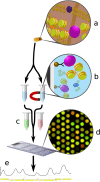
Figure 1. Representation of the ChIP-chip procedure.

Proteins are crosslinked to chromatin (a) which is extracted, sonicated and split into two samples. IP is carried out on one sample to separate out the chromatin bound to the factor of interest (b). Both samples are purified to DNA, amplified by PCR and differentially labelled (c). They are allowed to hybridise to the microarray probes and the resulting intensity values from the scanned image (d) are converted to numerical values which can be plotted (e) and processed as required by the investigation. Figure created and drawn by Mark Bennett.

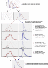
Figure 2. Representation of the normalisation procedure.

(a) Raw density profiles of datasets from two experimental conditions (red and blue), each with three replicates. Differences in the shapes of the profiles indicate experimentally induced biologically relevant changes, but these cannot be compared in their raw state. (b) Quantile normalising all datasets together (i) removes much of the experimentally induced, biologically relevant differences between them. This is not desirable, as these differences cannot then be investigated. Sandcastle quantile normalises the datasets from each experimental condition separately, to maintain these biological differences. Quantile normalisation makes each of the datasets follow the same distribution, meaning all density profiles from each experimental condition overlap each other (ii). This reduces intra-condition – but not inter-condition – technical variations. (c) Each dataset consists of two overlapping sub-populations (dashed lines), background (BG) and enriched (EN). These cannot be fully discerned in the data and only the overall population (solid lines) is known. Sandcastle performs inter-condition normalisation based on estimated background sub-populations. This requires the central (modal) point of the background sub-populations to be identifiable (marked with triangles). If this central point cannot be discerned (for example, if the background sub-population is too small) then the Sandcastle normalisation cannot be applied. (d) Data are first shifted to centre the modal point of the estimated background sub-population on zero (indicated by arrows). (e) To estimate the properties of the whole background sub-population all negative values (the left-hand side of the estimated background sub-population following the shift step) are mirrored into the positive (indicated by arrow; dashed lines show mirrored data). This allows the standard deviation of the estimated background sub-population to be calculated. (f) Data are scaled to the make the calculated standard deviation of the estimated background sub-population 1 (indicated by arrows). (g) The resulting fully normalised datasets have estimated background sub-populations with the same mean (0) and standard deviation (1). Comparisons of data between conditions can now be made relative to this common background. For clarity axis labels are only shown in (a) - all other x- and y-axes are ratio and density values respectively. Vertical grey lines indicate 0, which are only labelled in (f).

Figure 3. Enrichment and peak detection processes.

Two replicate datasets (coloured lines) and their average (black line) are represented along with the probe positions (coloured boxes). The cut-off value calculated for the particular dataset is shown (dashed line). All probes with all values above this cut-off are identified in the first stage of the enrichment detection procedure (highlighted probes). Windows around these probes are analysed (demonstrated with grey boxes for one probe in box (a)) to determine which, if any, windows contain probes deemed to be enriched over the whole window region. The first window extends upstream from the probe being analysed (as indicated by the arrow). The next window extends upwards from the furthest probe in this window, but not including it (as indicated by the arrow), and this process is repeated for all probes until the initial identified probe is reached. In this way all possible windows are identified for analysis. If the initial probe is found to be in any enriched window it is returned as an enriched probe by the software, whereas if it is not found to be in any enriched window it is not. If peak detection is required, averaged data are used to identify all maxima within the enriched probes (black crosses), each of which is returned as one peak. Maxima within individual datasets are also identified (coloured crosses) which are used to calculate potential binding regions of each peak (PBRs; demonstrated for one peak in box (b)). The PBR represents the region most likely to contain the binding site of the factor of interest and is defined as half the distance from the maxima to the next probe, up- and downstream of the maxima, unless this is distance is greater than the average chromatin shear size, in which case the distance is set to the average chromatin shear size. Peaks where all maxima fall at the same probe (as ‘i’) will therefore have narrower PBRs than those where they fall at adjacent probes (as ‘iii’). If all probe values are not above the cut-off (as ‘ii’ and ‘iv’) they are not identified as being enriched.

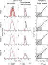
Figure 4. Examples of how the normalisation procedure affects real ChIP-chip datasets.

Data following each stage of the procedure are shown on each line (raw data, quantile normalisation applied, pseudo-modal shift applied, scaling applied). The first column shows all untreated (black line) and UV treated (red line) H3Ac binding datasets. Following the quantile normalisation step the replicate datasets follow the same overlapping distributions, hence only two visible lines. The second column shows a selected single untreated H3Ac dataset (black line) along with data mirrored about the zero point (red dashed line) and the SND over this same range (blue dotted line). The third column shows the same data as Q-Q plots, along with the position of the SND (blue dotted line), with data points below zero highlighted (grey box). These graphs show the estimated background region of the fully normalised data closely match the SND. All density plot x- and y-axes show ratio and density values respectively. All Q-Q plot x- and y-axes show theoretical and sample quantiles respectively.

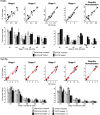
Figure 5. Validating the microarray normalisation procedure with Q-PCR.

6 H3Ac (top) and 5 Gcn5p (bottom) sites were examined with Q-PCR. For each normalisation stage (Stage 1 — Stage 4) a comparison between the microarray and Q-PCR data was made. Additionally all datasets were quantile normalised as one (Quantile Normalised). For each analysis Q-PCR data values were scaled to the microarray data values. Arrows represent 2 data points, from 2 experimental conditions, with the head of the arrow marking the second condition. The Gcn5p data shows arrows for untreated to time point 1 (t1; black) and time point 1 to time point 2 (t2; red). The angle of the arrows relative to the line y = x shows the similarity of the change between experimental conditions recorded by the two technologies, with angles close to this angle representing similar changes in both technologies. The distance of the points from the line y = x represents the similarity of values between the two technologies, with points closer to the line having more similar values. Bar charts show Q-PCR (shaded) and microarray (unshaded) values in preprocessed (Stage 1) and fully normalised (Stage 4) datasets for untreated (white) and treated (black, H3Ac; grey and black, Gcn5p) datasets. Error bars show standard errors.

Figure 6. Performance of the Sandcastle EDM on simulated datasets.

ROC-like curves showing the performance of the Sandcastle EDM at detecting simulated peaks in datasets with varying background distributions (data from a normal distribution, (a) T-distributions, (b,c) chi-squared distributions, (d,e)). y-axes show the proportion of true positives correctly identified and x-axes show the proportion of false positive results as a proportion of the number of true positives, such that the best possible results would lie in the top-left corners of the plots. Full calculation details are shown in the Methods section ‘ROC-like curves’. Coloured lines show the analysis of different numbers of datasets with results from varying FP values, each being the average of 50 simulations. Dots show the default FP value of 0.9. Increased performance is achieved when analysing multiple replicate datasets together than by analysing them individually. Even when simulating background distributions that violate the assumptions of the EDM the performance is still high. Results shown here are from data simulated with a degree of dependence between probe values in the same region, as may be expected in real data. Further plots are shown in Supplementary Figures S13–15.

Figure 7. Comparison of Sandcastle with ChIPOTle.

ROC-like curves showing the results of Sandcastle peak detection (black lines) compared with ChIPOTle peak detection (green and red lines) in data with background sub-populations simulated with data from normal (a), T- (5 degrees of freedom; (b)) and chi-squared (5 degrees of freedom; (c)) distributions. y-axes show the proportion of true positives correctly identified and x-axes show the proportion of false positive results as a proportion of the number of true positives, such that the best possible results would lie in the top-left corners of the plots. Full calculation details are shown in the Methods section ‘ROC-like curves’. For the normally distributed datasets (a) ChIPOTle was run with options assuming a Gaussian distribution (green lines) and the default option of using a peak height cut-off (red lines). The other distributions (b,c) were run using only the peak height cut-off option (red lines). For all tests it can be seen that Sandcastle outperforms ChIPOTle, as the results lie closer to the top-left corners of the plots.

References

1. Ren B. et al. Genome-wide location and function of DNA binding proteins. Science 290, 2306 (2000). - PubMed
1. Bernstein B. et al. Methylation of histone H3 Lys 4 in coding regions of active genes. P Natl Acad Sci USA 99, 8695 (2002). - PMC - PubMed
1. Pokholok D. et al. Genome-wide map of nucleosome acetylation and methylation in yeast. Cell 122, 517–527 (2005). - PubMed
1. Lee W. et al. A high-resolution atlas of nucleosome occupancy in yeast. Nat Genet 39, 1235–1244 (2007). - PubMed
1. Teng Y. et al. A novel method for the genome-wide high resolution analysis of DNA damage. Nucleic Acids Res 39, e10 (2011). - PMC - PubMed
Publication types
LinkOut - more resources