Estimation of noise properties for TV-regularized image reconstruction in computed tomography

Abstract

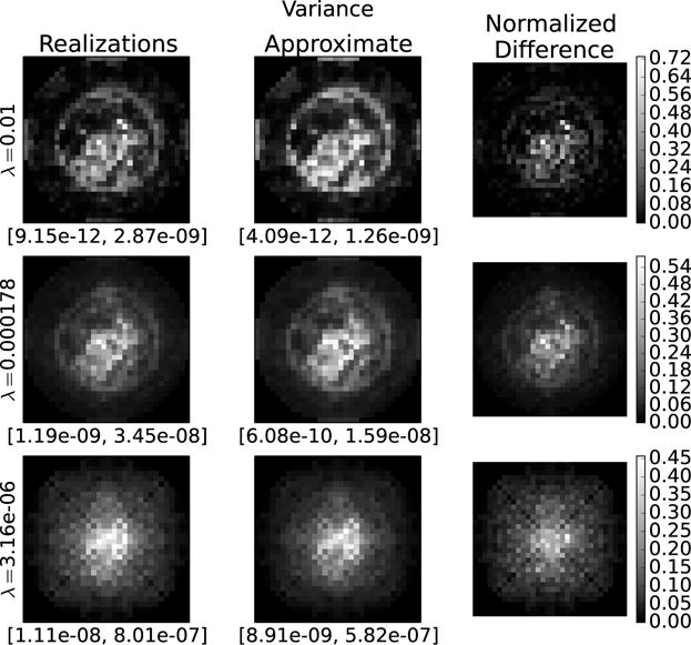
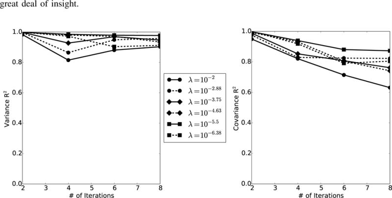
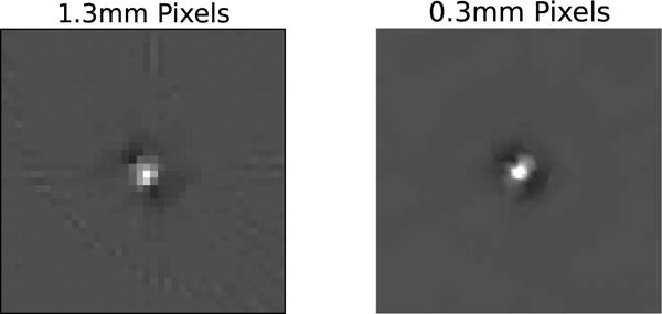
A method for predicting the image covariance resulting from total-variation-penalized iterative image reconstruction (TV-penalized IIR) is presented and demonstrated in a variety of contexts. The method is validated against the sample covariance from statistical noise realizations for a small image using a variety of comparison metrics. Potential applications for the covariance approximation include investigation of image properties such as object- and signal-dependence of noise, and noise stationarity. These applications are demonstrated, along with the construction of image pixel variance maps for two-dimensional 128 × 128 pixel images. Methods for extending the proposed covariance approximation to larger images and improving computational efficiency are discussed. Future work will apply the developed methodology to the construction of task-based image quality metrics such as the Hotelling observer detectability for TV-based IIR.

Fig. 1

The noise level used for validation is illustrated qualitatively in these reconstructed images with five values of regularization parameter λ, each reconstructed using 10 iterations of IRLS. These images are from separate noise realizations and correspond to the five regularization parameter strengths used in the evaluation below. The image on the far right is the numerical phantom used. The display window is [0.17, 0.25] cm⁻¹.

Fig. 2

Variance images from three different regularization parameter strengths. The display window of each image is given in the figure. The display windows are different so that the structure of the variance map estimate can be assessed. The right column provides the difference image between our approximation and the sample covariance from realizations, normalized to the maximum sample variance.

Fig. 3

Individual rows from the covariance matrices for three regularization parameter values. These rows had the worst RMSE between the two matrices of any rows, so they are the worst case approximations for each regularization strength. The color scale for the difference image is in % of the maximum covariance (i.e. percentage of the variance of the pixel corresponding to the row being visualized).

Fig. 4

The normalized RMSE between the approximated covariance matrix and the covariance matrix derived from realizations for the 32×32 image is shown for a range of regularization parameters including only the variance terms (left) and including all of the covariance terms (right). In this and subsequent figures, error bars arising from the statistical uncertainty of the sample covariance estimates are too small to be seen.

Fig. 5

Coefficients of determination R² for the variances and covariances between the approximation method and noise realizations.

Fig. 6

The regression metric ${\tilde{R}}^2$ with a model of equality between the approximation and the sample covariance is illustrated here as a function of regularization parameter and iteration. Results are shown for the variances alone (Left) as well as for the full covariance matrix (Right).

Fig. 7

The covariance distance metric, which is independent of matrix inversion, for a range of regularization parameters (left) and noise levels (right).

Fig. 8

Top: The two numerical phantoms used in this study, a numerical breast phantom (left), and a disk phantom (right). The display windows are [0.17, 0.25] cm⁻¹ and [0.17, 0.35] cm⁻¹, respectively. Arrows indicate the locations where local noise properties are studied in subsequent sections. Middle: Reconstructed noise realizations generated using the same phantoms. The display windows are identical to the images in the top row. Although heavy regularization is applied, some noise is still visible in the uniform regions of the phantoms. Bottom: Difference images between two noisy IRLS reconstructions of each phantom are shown in order to visualize the noise structure. The display windows are [−0.001, 0.001] cm⁻¹ and [−0.003, 0.003] cm⁻¹ for the left and right images, respectively.

Fig. 9

Shown here are difference images between two independent noise realizations. On the left, the two images have been reconstructed using 6 iterations of the IRLS algorithm. On the right, the same data realizations were propagated through the linearization of Eqn. 30. The patchy noise structure which is evident in the IRLS reconstructions is well preserved in the linearization approach, meaning that the characteristic noise texture of TV minimization can potentially be well approximated with only 2nd-order image statistics. As in the small system examples, note that the noise magnitude appears to be the primary source of error in the linear approximation.

Fig. 10

Variance maps for each phantom determined by approximation method. The display window in each case is [0, 2×10⁻⁶] cm⁻². Note the strong noise dependene on local edge information, as previously reported by others [30], [58].

Fig. 11

Correlation structure in the breast phantom (top) and the disk phantom (bottom) for the two phantom locations indicated in Figure 8. The display window of each image is set so that white corresponds to 50% of the maximum covariance and the gray level of 0 is kept constant. Differences between the two rows illustrate the object-dependence of the noise structures in images reconstructed with TV minimization. In general, any IIR approach potentially produces object-dependent noise. Additionally, comparison between the two columns illustrates the degree of global non-stationarity of the image noise.

Fig. 12

Each image shows the correlation structure in a region of the breast phantom reconstruction near a tissue boundary. The left image is centered on the boundary pixel in Figure 13. The right image is centered on a point slightly to the right of the left image’s center. The distance between the two points is only 4 pixels, but non-stationarity is clearly evident through the change in the correlation structure. The display window is [−2×10⁻⁸, 4×10⁻⁸] cm⁻² for both figures.

Fig. 13

Shown are the resulting vectors ${\tilde{e}}_i$ from Eqn. 36, reshaped into 2-dimensional images. The existence of many pixels which are non-zero is a direct indication that the DFT does not diagonalize the image covariance matrix, hence invalidating the assumption of stationarity. The display window is set so that black corresponds to 0, while white corresponds to 25% of the maximum image value.

Fig. 14

These results, similar to those in Figure 13, demonstrate that local stationarity is similarly not satisfied, despite restriction of the image ROI to small sizes. The headings of the figures denote the width of the square ROI used. The window for each image is set as in Figure 13.

Fig. 15

In order to demonstrate the feasibility of computing covariance estimates for large images, 200 noise realizations were used to construct an estimate of ${\overline{\mathbf{w}}}_n$ for a 512 × 512 pixel image at the same off-center pixel location in the breast phantom as in Figure 11. The method of conjugate gradients was then used to solve the linear systems in Algorithms 1 and 2.

References

1. Sidky EY, Kao C-M, Pan X. Accurate image reconstruction from few-views and limited-angle data in divergent-beam CT. Journal of X-ray Science and Technology. 2006;14(2):119–139.
1. Sidky EY, Pan X. Image reconstruction in circular cone-beam computed tomography by constrained, total-variation minimization. Physics in medicine and biology. 2008;53(17):4777. - PMC - PubMed
1. Defrise M, Vanhove C, Liu X. An algorithm for total variation regularization in high-dimensional linear problems. Inverse Problems. 2011;27(6):065002.
1. Jensen TL, Jrgensen JH, Hansen PC, Jensen SH. Implementation of an optimal first-order method for strongly convex total variation regularization. BIT Numerical Mathematics. 2012;52(2):329–356.
1. Jorgensen JS, Sidky EY, Pan X. Quantifying admissible undersampling for sparsity-exploiting iterative image reconstruction in x-ray CT. Medical Imaging, IEEE Transactions on. 2013;32(2):460–473. - PMC - PubMed
Publication types