

Predicting cortical bone adaptation to axial loading in the mouse tibia
- PMID: 26311315
- PMCID: PMC4614470
- DOI: 10.1098/rsif.2015.0590
Predicting cortical bone adaptation to axial loading in the mouse tibia
Abstract
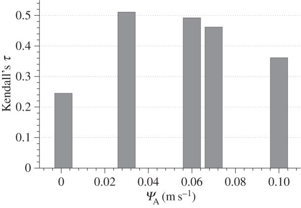
The development of predictive mathematical models can contribute to a deeper understanding of the specific stages of bone mechanobiology and the process by which bone adapts to mechanical forces. The objective of this work was to predict, with spatial accuracy, cortical bone adaptation to mechanical load, in order to better understand the mechanical cues that might be driving adaptation. The axial tibial loading model was used to trigger cortical bone adaptation in C57BL/6 mice and provide relevant biological and biomechanical information. A method for mapping cortical thickness in the mouse tibia diaphysis was developed, allowing for a thorough spatial description of where bone adaptation occurs. Poroelastic finite-element (FE) models were used to determine the structural response of the tibia upon axial loading and interstitial fluid velocity as the mechanical stimulus. FE models were coupled with mechanobiological governing equations, which accounted for non-static loads and assumed that bone responds instantly to local mechanical cues in an on-off manner. The presented formulation was able to simulate the areas of adaptation and accurately reproduce the distributions of cortical thickening observed in the experimental data with a statistically significant positive correlation (Kendall's τ rank coefficient τ = 0.51, p < 0.001). This work demonstrates that computational models can spatially predict cortical bone mechanoadaptation to a time variant stimulus. Such models could be used in the design of more efficient loading protocols and drug therapies that target the relevant physiological mechanisms.
Keywords: bone mechanobiology; cortical thickness; fluid flow; functional adaptation; mouse tibia.
© 2015 The Authors.
Figures
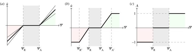
 (mechanical stimulus versus adaptation) relationship curves considered in this study: (a) generic trilinear curve, (b) trilinear curve capped with maximum remodelling rates of apposition and resorption, (c) on–off relationship. The apposition and resorption limits of the homeostatic interval, ΨA and ΨR, dictate the tissue response to mechanical stimulus Ψ. The step curve in (c) obtained the most accurate predictions of cortical adaptation.
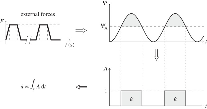
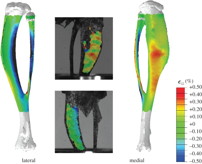
 calculated in the FE models and DIC measurements in eight-week-old mice of the same strain and gender by Sztefek et al. [34]. FEA used the geometry of a non-adapted tibia under an axial peak load of 12 N. (DIC images adapted from [34] with permission from Elsevier.)
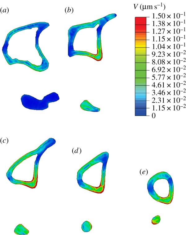
References
-
- Frost HM. 1964. The laws of bone structure. Springfield, IL: Charles C. Thomas.
-
- Cavanagh PR, Licata AA, Rice AJ. 2005. Exercise and pharmacological countermeasures for bone loss during long-duration space flight. Gravit. Space Biol. Bull. 18, 39–58. - PubMed
-
- Issekutz B, Blizzard JJ, Birkhead NC, Rodahl K. 1966. Effect of prolonged bed rest on urinary calcium output. J. Appl. Physiol. 21, 1013–1020. - PubMed
-
- Haapasalo H, Kontulainen S, Sievänen H, Kannus P, Järvinen M, Vuori I. 2000. Exercise-induced bone gain is due to enlargement in bone size without a change in volumetric bone density: a peripheral quantitative computed tomography study of the upper arms of male tennis players. Bone 27, 351–357. ( 10.1016/S8756-3282(00)00331-8) - DOI - PubMed
Publication types
MeSH terms
Grants and funding
LinkOut - more resources
Full Text Sources
Other Literature Sources