Dopamine neurons projecting to the posterior striatum form an anatomically distinct subclass

Abstract

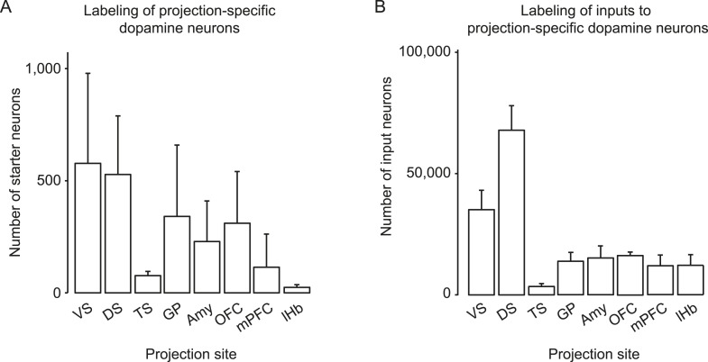
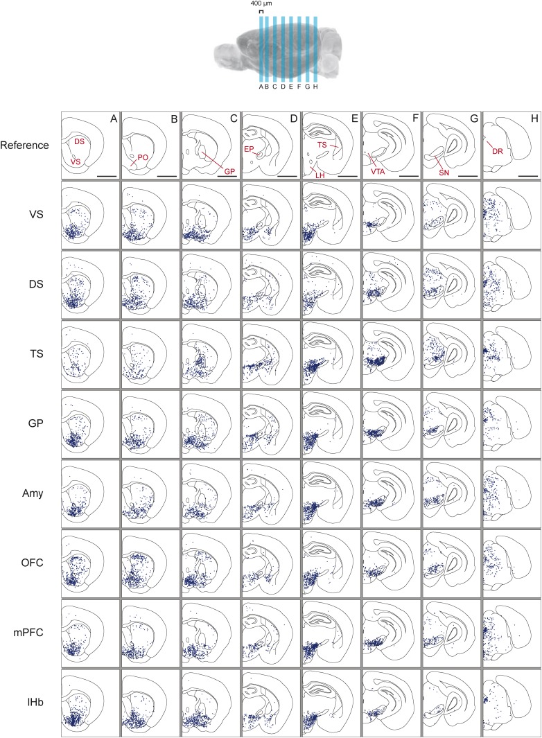
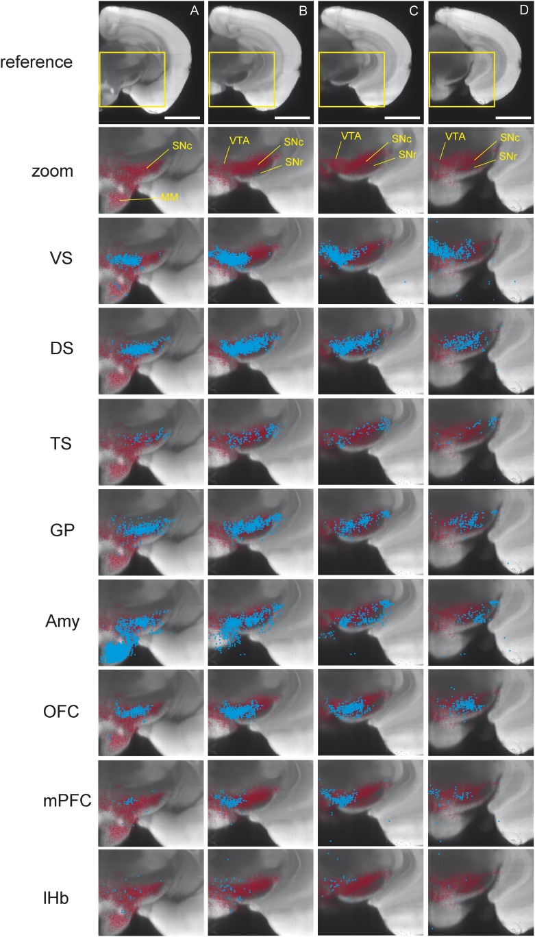
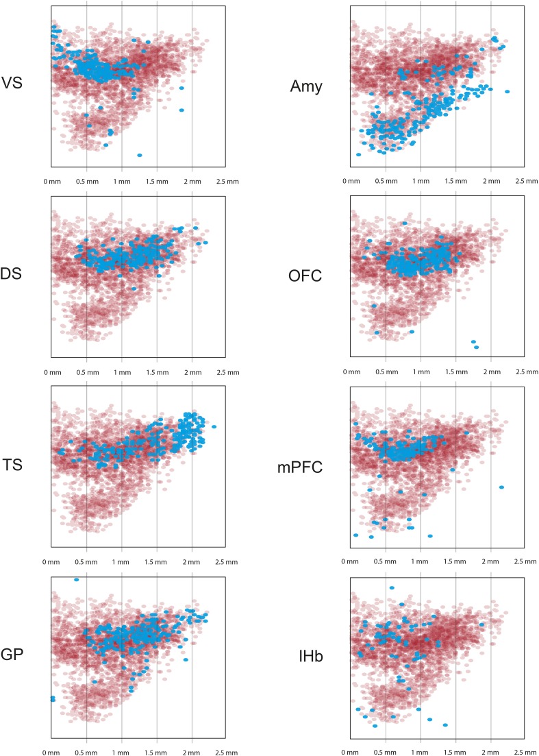
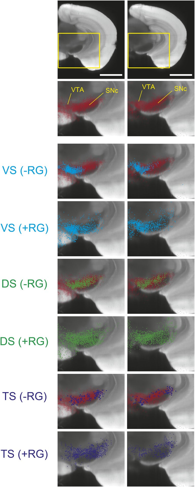
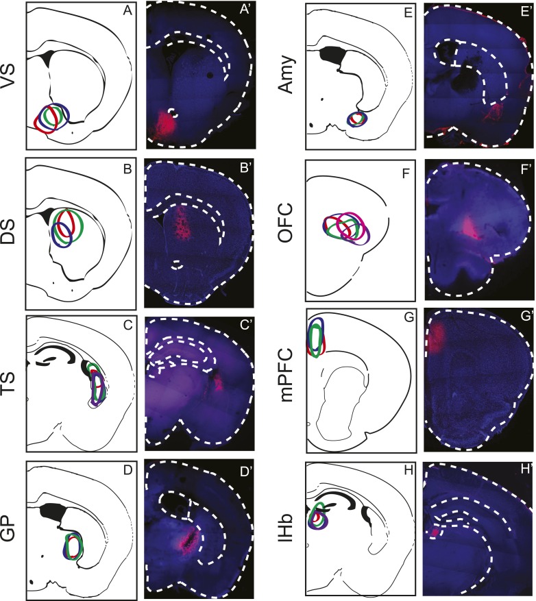
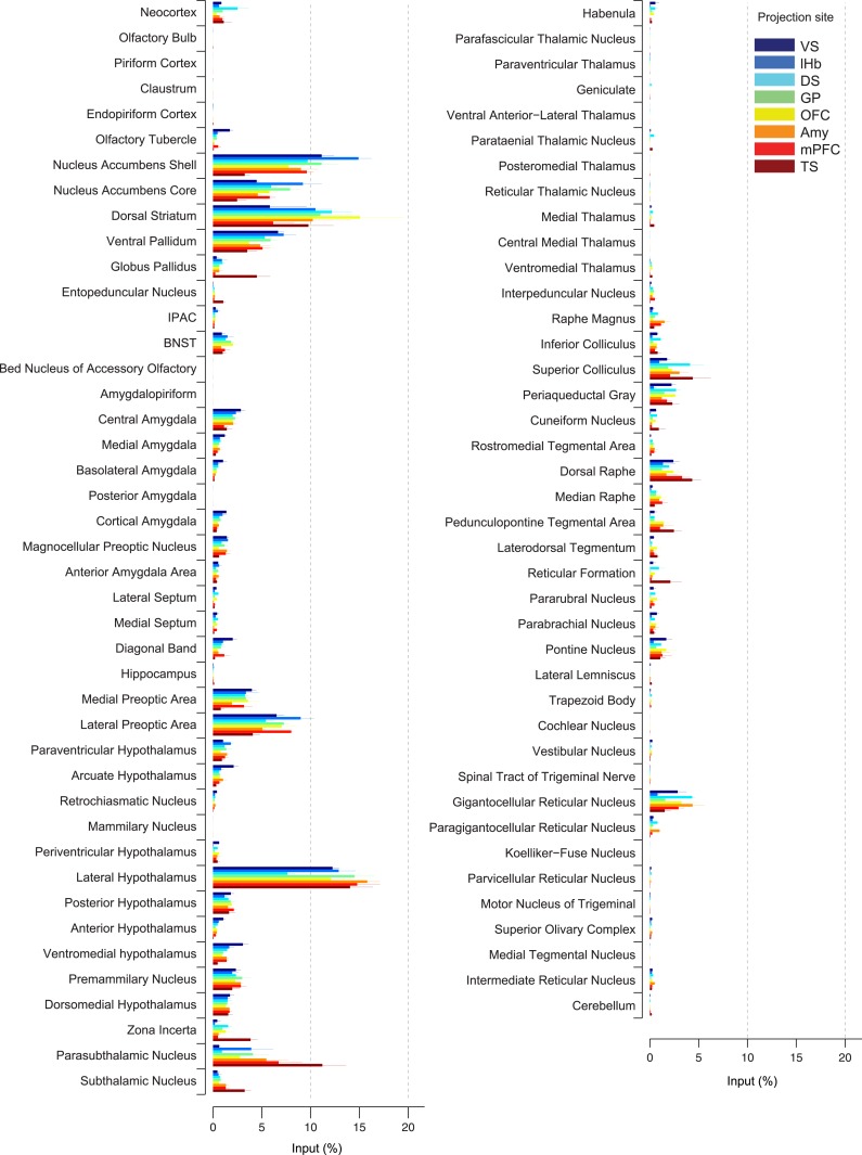
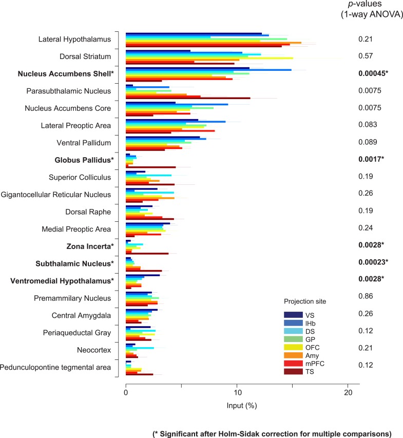
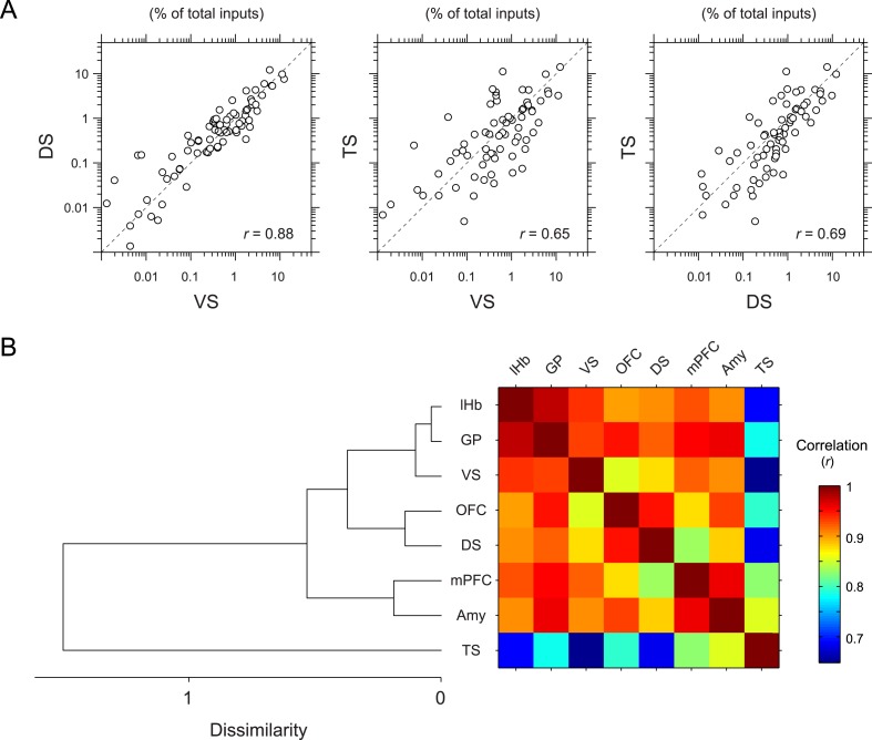
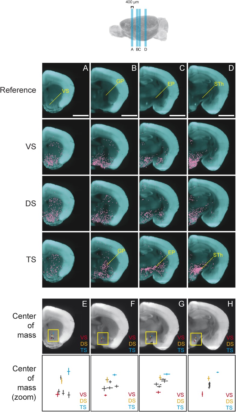
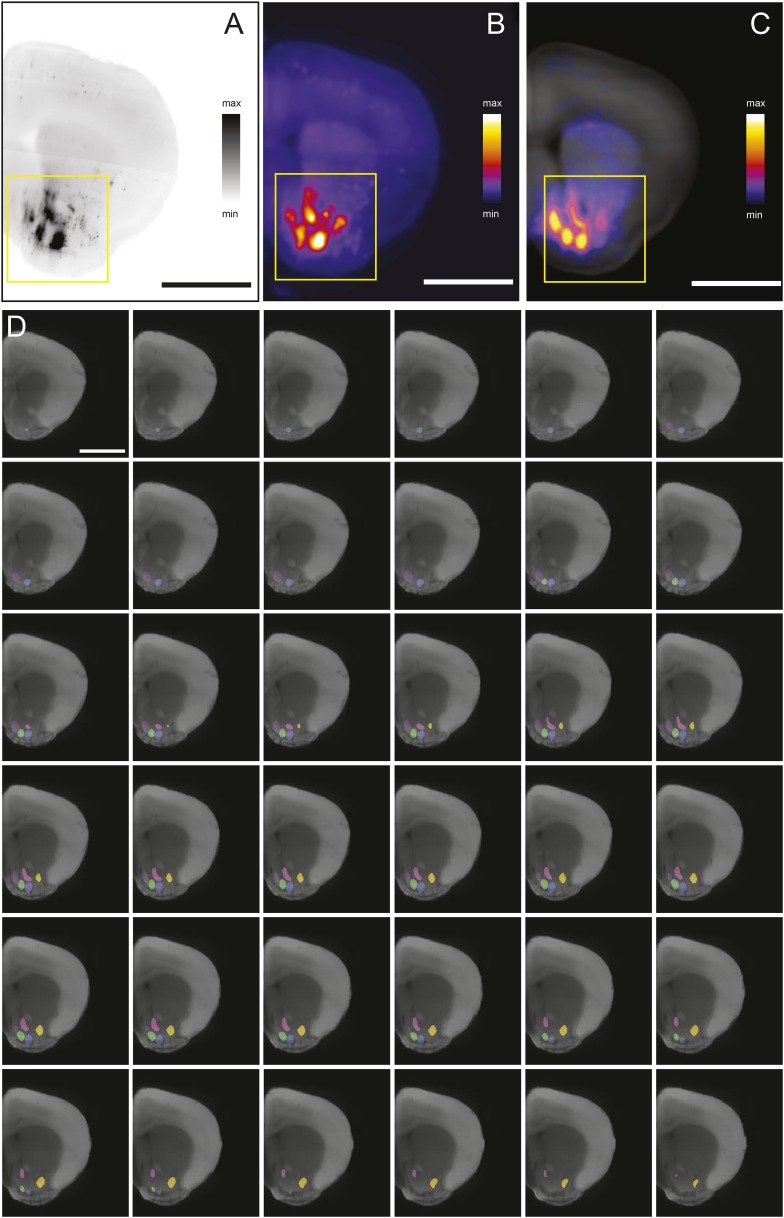
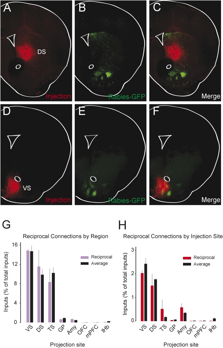
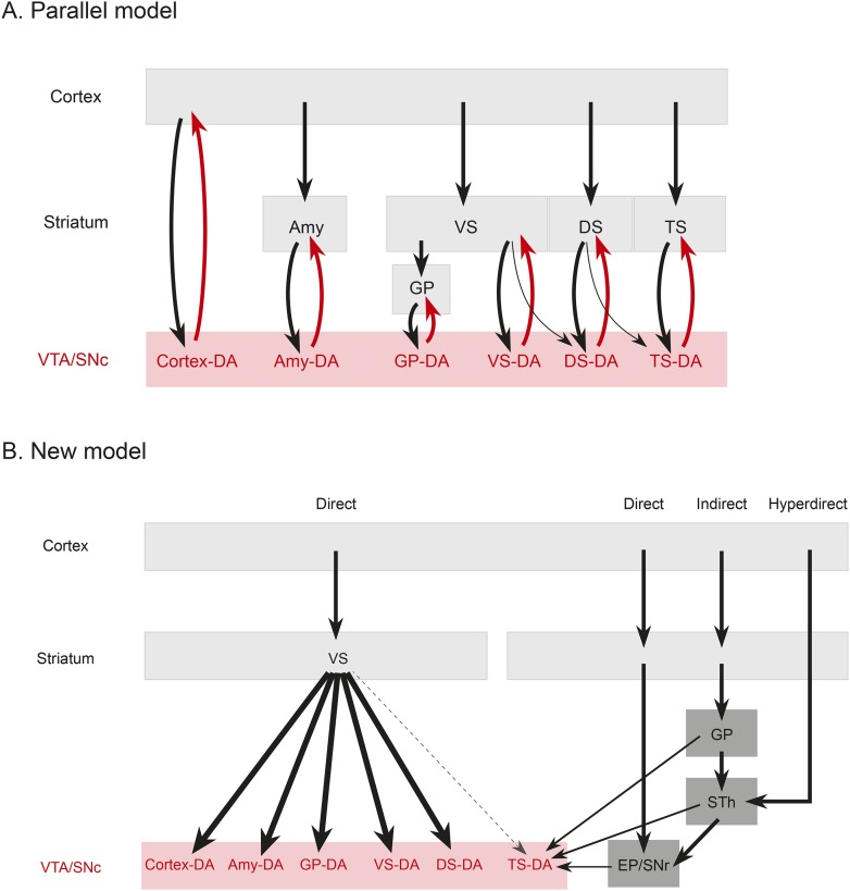
Combining rabies-virus tracing, optical clearing (CLARITY), and whole-brain light-sheet imaging, we mapped the monosynaptic inputs to midbrain dopamine neurons projecting to different targets (different parts of the striatum, cortex, amygdala, etc) in mice. We found that most populations of dopamine neurons receive a similar set of inputs rather than forming strong reciprocal connections with their target areas. A common feature among most populations of dopamine neurons was the existence of dense 'clusters' of inputs within the ventral striatum. However, we found that dopamine neurons projecting to the posterior striatum were outliers, receiving relatively few inputs from the ventral striatum and instead receiving more inputs from the globus pallidus, subthalamic nucleus, and zona incerta. These results lay a foundation for understanding the input/output structure of the midbrain dopamine circuit and demonstrate that dopamine neurons projecting to the posterior striatum constitute a unique class of dopamine neurons regulated by different inputs.

Keywords: anatomy; dopamine; input; monosynaptic; mouse; neuroscience; rabies virus; striatum.

Figure 1.. Labeling projection-specific dopamine neurons and their monosynaptic inputs throughout the brain with rabies-GFP.

(A) A schematic of the injections used to label projection-specific populations of dopamine neurons. The blue circle represents the site of infection with adeno-associated virus (AAV)-FLEX-TVA and green neurons represent the DAT-Cre-expressing dopamine neurons projecting to that area. (B) Horizontal optical section showing rabies-GFP signal following AAV-FLEX-TVA injection into the striatum of a DAT-Cre animal followed by rabies injection into the ventral tegmental area (VTA) and substantia nigra pars compacta (SNc). The numbers of infected neurons are shown in Figure 1—figure supplement 1. Bar indicates 2 mm. (C) Coronal physical section showing rabies labeled neurons from (B) in green and anti-TH antibody staining in red. Bar indicates 500 μm. (D–F) Higher magnification image of rabies labeled neurons and tyrosine hydroxylase (TH) staining. Bars indicate 200 μm. (G) A schematic of the injections used to label the inputs of projection-specific populations of dopamine neurons throughout the brain. The blue circle represents the site of infection with AAV-FLEX-TVA and the red circle represents the site of infection with AAV-FLEX-RG. Green neurons outside of VTA/SNc represent the monosynaptic inputs labeled throughout the brain. (H) Horizontal optical section showing rabies-GFP signal following AAV-FLEX-TVA injection into the striatum and AAV-FLEX-RG into the VTA and SNc of a DAT-Cre animal followed by rabies injection into the VTA and SNc. Number of infected neurons shown in Figure 1—figure supplement 1. Bar indicates 2 mm. DOI: http://dx.doi.org/10.7554/eLife.10032.003

Figure 1—figure supplement 1.. Number of starter cells and inputs labeled.

(A) The average numbers of projection-specified dopamine neurons labeled in each condition, using the injection schematic shown in Figure 1A with the indicated injection sites of AAV-FLEX-TVA on the x-axis of the graph. Mean ± s.e.m. (B) The average numbers of inputs (outside of the VTA/SNc) labeled in each condition using the injection schematic shown in Figure 1H with the indicated injection sites of AAV-FLEX-TVA on the x-axis of the graph. Mean ± s.e.m. DOI: http://dx.doi.org/10.7554/eLife.10032.004

Figure 2.. Automated acquisition and analysis of whole-brain tracing data.

(A) A schematic of the brain clearing, imaging, and analysis pipeline used to acquire data from brains labeled using the injection schematics outlined in Figure 1A and Figure 1G. (B) A graphical explanation of the image acquisition and stitching process. Whole brains were imaged horizontally, from the dorsal (orange arrow) and ventral (purple arrow) sides and these images were stitched and combined to create a whole brain image. An example brain expressing tdTomato under the control of genetically encoded Vglut2-Cre is shown. (C) An example of a horizontal optical section acquired as described in A, B. Boxes indicate the locations of inset panels. Bar indicates 2 mm. (D) The automatically generated segmentation of C, with each labeled cell being represented by a single pixel. Bar indicates 2 mm. (E–H) Insets displaying raw images and automatically generated segmentations from the indicated regions (cortex, striatum, midbrain, and cerebellum). Bars indicate 200 μm. DOI: http://dx.doi.org/10.7554/eLife.10032.005

Figure 3.. Distribution of monosynaptic inputs to projection-specific populations of dopamine neurons throughout the brain.

A summary of the inputs to each of the projection-specified populations of dopamine neurons assayed (using the injection scheme from Figure 1G) normalized such that the 1500 neurons were randomly sampled from each brain. We then combined such subsampled neurons from three randomly selected animals for each condition and plotted them in corresponding 400 μm sections. Inputs to: VS-projecting, DS-projecting, TS-projecting, GP-projecting, Amy-projecting, OFC-projecting, mPFC-projecting, and lHb-projecting dopamine neurons as well as selected coronal sections for reference (A–H). In this figure, and all others, the following abbreviations were used: ‘VS’ for ventral striatum, ‘DS’ for anterior dorsal striatum, ‘TS’ for tail of the striatum (posterior striatum), ‘GP’ for globus pallidus, ‘Amy’ for amygdala, ‘OFC’ for orbitofrontal cortex, ‘mPFC’ for medial prefrontal cortex, and ‘lHb’ for lateral habenula. Data collected in the same manner from experiments with no transsynaptic spread shown in Figure 3—figure supplement 1 and Figure 3—figure supplement 2, comparison of the two conditions shown in Figure 3—figure supplement 3, and injection sites used shown in Figure 3—figure supplement 4 and Figure 3—figure supplement 5. Bars indicate 2 mm. DOI: http://dx.doi.org/10.7554/eLife.10032.006

Figure 3—figure supplement 1.. Distribution of projection-specific populations of dopamine neurons within the midbrain.

A summary of the projection-specified populations of dopamine neurons labeled (using the injection scheme from Figure 1A) in cyan, compared to the distribution of all DAT-cre expressing neurons in the area of the injection in red. Distribution of: VS-projecting dopamine neurons, DS-projecting dopamine neurons, TS-projecting dopamine neurons, GP-projecting dopamine neurons, Amy-projecting dopamine neurons, OFC-projecting dopamine neurons, mPFC-projecting dopamine neurons, lHb-projecting dopamine neurons, and selected landmarks for reference (A–D). Plots were prepared by projecting all neurons within 400 μm of the selected coronal plane onto a single image. Bars represent 2 mm. DOI: http://dx.doi.org/10.7554/eLife.10032.007

Figure 3—figure supplement 2.. Distribution of projection-specific populations of dopamine neurons within the midbrain: Maximum Intensity Projection.

For each graph, 75 neurons were sampled at random from 3 of the (−RG) brains shown in Figure 3—figure supplement 1. These 225 neurons were then plotted as a ‘maximum intensity projection’ (i.e., their Z coordinate was ignored). In the case of Lhb-projecting dopamine neurons, labeling was very sparse, so we plotted all 122 neurons. The distribution of all DAT-cre expressing neurons is shown in red. The distribution of dopamine neurons projecting to the indicated site in each case is shown in cyan. Grid lines indicate 500 microns. DOI: http://dx.doi.org/10.7554/eLife.10032.008

Figure 3—figure supplement 3.. Comparison of labeled cell distribution between control and experimental groups.

A comparison of the distribution of labeled VTA/SN neurons in experiments lacking RG (labeling dopamine ‘starter neurons’ only) and experiments with RG (labeling dopamine ‘starter neurons’ as well as their monosynaptic inputs). Coronal planes match Figure 3—figure supplement 1B,C. VS, DS, and TS are color-coded, while the total distribution of all DAT-Cre expressing neurons in the area are shown in red. DOI: http://dx.doi.org/10.7554/eLife.10032.009

Figure 3—figure Supplement 4.. Injection Sites.

CLARITY-based brain clearing did not preserve native BFP fluorescence, so brains were physically sectioned and stained with an anti-BFP antibody to label the injection site of AAV-FLEX-TVA in each animal. All injection sites used for input tracing (based on the schematic in Figure 1G) are summarized in the left panels and a single raw image from each is displayed in the panels on the right. Injection sites were intended to allow TVA uptake into VS-projecting (A–A′), DS-projecting, (B–B′), TS-projecting (C–C′), GP-projecting (D–D′), Amy-projecting (E–E′), OFC-projecting (F–F′), mPFC-projecting (G–G′), and lHb-projecting (H–H′) dopamine neurons. Red: injection sites. Blue: autofluorescence. DOI: http://dx.doi.org/10.7554/eLife.10032.010

Figure 3—figure supplement 5.. Subdivisions of the striatum.

(A) Maximum intensity projection (horizontal) of the outline of the brain (black), the DS (green), the nucleus accumbens (orange), and the injections into VS (blue), DS (cyan), and TS (red). Stereotactic coordinates are shown as grid lines with 1 mm spacing. (B) Maximum intensity projection (sagittal) of the outline of same injection sites as shown in above. (C) Coronal views of the approximate centers of the VS/DS and TS injections. DOI: http://dx.doi.org/10.7554/eLife.10032.011

Figure 4.. Comparison of the percentage of inputs from each region across populations of projection-specific dopamine neurons.

A summary of the distribution of inputs to dopamine neurons with different projection sites, with bars representing the average % of inputs observed (out of all labeled input neurons outside of the VTA/SNc/SNr/RRF) per region (mean ± s.e.m.). Each color represents inputs to a different population of dopamine neurons, as indicated in the inset. The 20 most prominent inputs are compared in Figure 4—figure supplement 1. DOI: http://dx.doi.org/10.7554/eLife.10032.012

Figure 4—figure supplement 1.. Comparison of the percentage of inputs from selected regions across populations of projection-specific dopamine neurons.

A summary of the distribution of inputs among the 20 most prominent regions providing input to dopamine neurons. These areas were selected based on the maximum percentage of inputs among eight conditions for each area. Plots are identical to those displayed in Figure 4 and each condition is labeled with the same color as in Figure 4. p-Values are given based on 1-way ANOVA. Asterisks (*) indicate significant differences among conditions after Holm-Sidak corrections for multiple comparisons. DOI: http://dx.doi.org/10.7554/eLife.10032.013

Figure 5.. Correlation between projection-specific populations of dopamine neurons.

(A) Scatter plots comparing the percent of inputs from each anatomical region for VS-, DS-, and TS-projecting dopamine neurons. Each circle represents the average percent of inputs for one anatomical area for each condition. r: Pearson's correlation coefficient. The axes are in log scale. (B) Dendrogram (left) and correlation matrix (right) summarizing all pair-wise comparisons. Color on the right indicates correlation values. The dendrogram was generated based on hierarchical clustering using the average linkage function. DOI: http://dx.doi.org/10.7554/eLife.10032.014

Figure 6.. Topological shift in the center of mass of input neurons to projection-specified dopamine neurons.

Four coronal optical sections (400 μm thick) were chosen to demonstrate the dorsolateral shift of inputs to TS-projecting dopamine neurons. (A–D) Coronal optical sections, with a region of interest marked in yellow for reference. Bars represent 2 mm. The distribution of inputs to each population of neurons is plotted in magenta and neurons within the ventral striatum (A), GP (B), entopeduncular nucleus (EP) (C), and subthalamic nucleus (STh) (D) are indicated. A fixed number of neurons were randomly chosen from each brain and those neurons from three randomly chosen animals per condition were plotted for corresponding coronal sections. (E–H) Coronal optical sections, with a yellow box showing the location of the insets displayed below. The center of mass for each population is shown, with vertical and horizontal lines representing the standard error in the y-axis and x-axis, respectively. DOI: http://dx.doi.org/10.7554/eLife.10032.015

Figure 7.. Dense regions of inputs within the ventral striatum.

(A–C) Coronal optical sections showing typical distributions of inputs in the ventral striatum. A comparison of the typical ‘patch’ structure of inputs from the ventral striatum (to VS-projecting or DS-projecting dopamine neurons, for example) with the atypical ‘patch-less’ structure of inputs from the striatum to TS-projecting dopamine neurons. (D) Percentage of input neurons within the ventral striatum (core, medial shell, and lateral shell combined) in each condition. Red dotted line indicates the percentage expected based on chance distribution throughout the brain, while green dotted line indicates the average percentage among all animals. (E) Horizontal optical section showing a typical distribution of inputs in the ventral striatum, with many input neurons in tight clusters. Bar represents 2 mm. (F) A zoomed view of E, taken from the indicated box. Clusters are dispersed along the A-P axis, so two planes are used to display them in coronal sections: the black arrow indicates the anterior plane and the white arrow indicated the posterior plane. (G–H) Coronal optical sections showing the two planes indicated above, as well as a graphical representation of the five patches in those planes. (I) Among labeled neurons in the ventral striatum, the percentage within the patches in each condition. Red dotted line indicates the percentage expected based on chance distribution throughout the nucleus accumbens, while green dotted line indicates the average percentage among all animals. (J) Among labeled neurons within the patches, the percentages within each patch in each condition. Green arrows point to patch 2, cyan arrows point to patch 3, and yellow arrows point to patch 5. More detailed description of the patches shown in Figure 7—figure supplement 1. DOI: http://dx.doi.org/10.7554/eLife.10032.016

Figure 7—figure supplement 1.. Density-based analysis of inputs to projection-specified dopamine neurons.

All neurons from all animals were plotted in a reference space with 20 μm × 20 μm × 20 μm voxels, and a 3D Gaussian with kernel size of 60 μm × 60 μm × 60 μm was used to estimate density at each voxel. (A) A typical optical coronal section of raw fluorescence containing the ventral striatum colored such that black indicates fluorescence. (B) Average fluorescence among all animals displayed as a heat map. (C) Density estimate based on Gaussian smoothing of the image generated by plotting all extracted centroids from all animals displayed as a heat map. (D) A series of coronal sections demonstrating the 3D structure of the patches, obtained by finding the local maxima from C and expanding stepwise pixel-by-pixel until either 1/3 maximum intensity or another patch boundary was reached. Patch coloring matches Figure 7. Bars represent 2 mm. DOI: http://dx.doi.org/10.7554/eLife.10032.017

Figure 8.. Reciprocity of connection between dopamine neurons and neurons at their projection sites.

CLARITY-based brain clearing did not preserve native BFP fluorescence, so brains were physically sectioned and stained with an anti-BFP antibody to label the injection site of AAV-FLEX-TVA in each animal. (A–C) The injection site (red) and input neurons (green) labeled in a physical coronal section for DS-projecting dopamine neurons. (D–F) The injection site (red) and input neurons (green) labeled in a physical coronal section for VS-projecting dopamine neurons. (G) A comparison of the percentage of inputs from the reciprocal region (defined by brain region) of each injection site (in purple) with the average percentage of inputs from that region among all other brains (in black). For this analysis, the DS was split into ‘anterior DS’ for DS and ‘posterior DS’ for TS at Bregma −0.9 mm. There were no significant differences between pairs (two-sample t-test). (H) A comparison of the percentage of inputs from the reciprocal site (defined by region of BFP infection) of each injection (in red) with the average percentage of inputs from that region among all other brains (in black). There were no significant differences between pairs (two-sample t-test). DOI: http://dx.doi.org/10.7554/eLife.10032.018

Figure 9.. Summary and model.

(A) A working model suggesting that dopamine neurons receive inputs primarily from the region that they project to, based on the idea that input neurons provide an ‘expectation’ signal and dopamine neurons correct them (i.e., send them a prediction error signal based on the type of expectation that they encoded) individually. (B) Our model, in which dopamine neurons in the ‘canonical’ pathway receive inputs primarily from a common set of regions (and particularly heavy inputs from the ventral striatum) and send a common prediction error signal to many parts of the forebrain. We propose that TS-projecting dopamine neurons could be part of a relatively separate pathway with a potentially unique function (different from reward prediction error (RPE) calculation) based on its unique distribution of inputs. Some common inputs such as the DS and ventral pallidum are omitted for clarity. DOI: http://dx.doi.org/10.7554/eLife.10032.019

References

1. Alheid GF, Heimer L. New perspectives in basal forebrain organization of special relevance for neuropsychiatric disorders: the striatopallidal, amygdaloid, and corticopetal components of substantia innominata. Neuroscience. 1988;27:1–39. doi: 10.1016/0306-4522(88)90217-5. - DOI - PubMed
1. Backman CM, Malik N, Zhang Y, Shan L, Grinberg A, Hoffer BJ, Westphal H, Tomac AC. Characterization of a mouse strain expressing Cre recombinase from the 3′ untranslated region of the dopamine transporter locus. Genesis. 2006;44:383–390. - PubMed
1. Bayer HM, Glimcher PW. Midbrain dopamine neurons encode a quantitative reward prediction error signal. Neuron. 2005;47:129–141. doi: 10.1016/j.neuron.2005.05.020. - DOI - PMC - PubMed
1. Bayer VE, Pickel VM. Ultrastructural localization of tyrosine hydroxylase in the rat ventral tegmental area: relationship between immunolabeling density and neuronal associations. The Journal of Neuroscience. 1990;10:2996–3013. - PMC - PubMed
1. Beier KT, Steinberg EE, DeLoach KE, Xie S, Miyamichi K, Schwarz L, Gao XJ, Kremer EJ, Malenka RC, Luo L. Circuit architecture of VTA dopamine neurons revealed by systematic input-output mapping. Cell. 2015;162:622–634. doi: 10.1016/j.cell.2015.07.015. - DOI - PMC - PubMed