Bayesian hierarchical grouping: Perceptual grouping as mixture estimation

Abstract

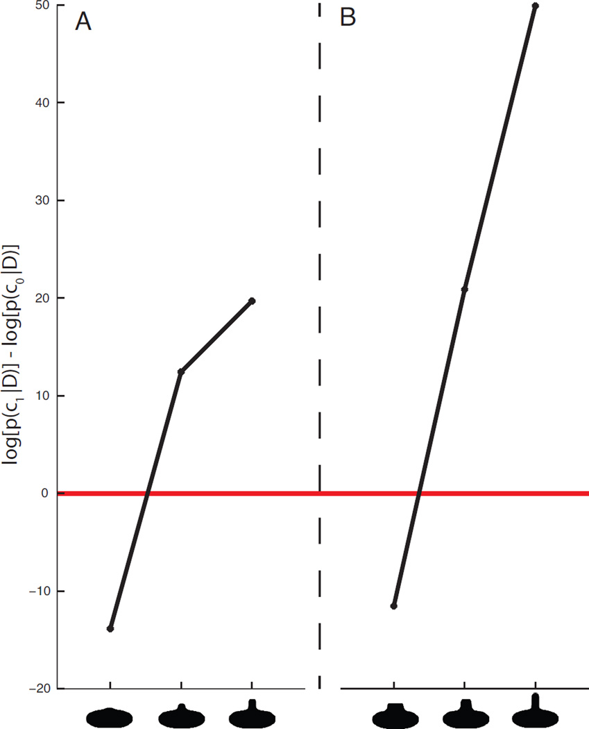
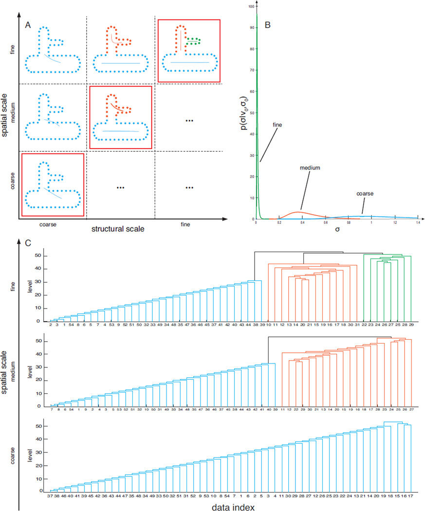
We propose a novel framework for perceptual grouping based on the idea of mixture models, called Bayesian hierarchical grouping (BHG). In BHG, we assume that the configuration of image elements is generated by a mixture of distinct objects, each of which generates image elements according to some generative assumptions. Grouping, in this framework, means estimating the number and the parameters of the mixture components that generated the image, including estimating which image elements are "owned" by which objects. We present a tractable implementation of the framework, based on the hierarchical clustering approach of Heller and Ghahramani (2005). We illustrate it with examples drawn from a number of classical perceptual grouping problems, including dot clustering, contour integration, and part decomposition. Our approach yields an intuitive hierarchical representation of image elements, giving an explicit decomposition of the image into mixture components, along with estimates of the probability of various candidate decompositions. We show that BHG accounts well for a diverse range of empirical data drawn from the literature. Because BHG provides a principled quantification of the plausibility of grouping interpretations over a wide range of grouping problems, we argue that it provides an appealing unifying account of the elusive Gestalt notion of Prägnanz.

Figure 1

Illustration of the Bayesian hierarchical clustering process. (A) Example tree decomposition (see also Heller & Ghahramani, 2005) for the 1D grouping problem on the right; (B) Tree slices, i.e. different grouping hypotheses. (C) Tree decomposition as computed by the clustering algorithm for the dot-clusters on the right, assuming bivariate Gaussian objects; (D) Tree slices for the dot-clusters.

Figure 2

The generative function of our model depicted as a field. Ribs sprout perpendicularly from the curve (red) and the length they take on is depicted by the contour plot. (A) For contours ribs are sprouted with a μ close to zero, resulting in a Gaussian fall-off along the curve. (B) For shapes ribs are sprouted with μ > 0 resulting in a band surrounding the curve.

Figure 3

BHG predictions for simple dot lattices. As input the model received the location of the dots as seen in the bottom two rows, where the ratio of the vertical |b| over the horizontal |a| dot distance was manipulated. The graphs on top shows the log posterior ratio of seeing vertical versus horizontal contours as a function of the ratio |b|/|a|. (left plot) Object definition included error on arclength; (right plot) Object definition included a quadratic error on arclength.

Figure 4

BHG’s performance on data from Feldman (2001). (A,B) Sample stimuli with likely responses (stimuli not drawn to scale). (C) Log odds of the pooled subject responses plotted as a function of the log posterior ratio of the model log p(c₂|D) − log p(c₁|D), where each point depicts one of the 343 stimulus types shown in the experiment. Both indicate the probability of seeing two contours p(c₂|D). Model responses are linearized using an inverse cumulative Gaussian.

Figure 5

The “association field” between two line segments (each containing 5 dots) as quantified by BHG. (A) Manipulation of the distance and angle between these two line segments. The blue line depicts the one-object hypothesis, and the two green lines depict the two-objects hypothesis. (B) The association field reflecting the posterior probability of p(c₁|D) of the one-object hypothesis.

Figure 6

BHG results for simple dot contours. The first column shows the input images and their MAP segmentation. Input dots are numbered from left to right. The second column shows the tree decomposition as computed by BHG. The third column shows the posterior probability distribution over all tree-consistent decompositions (i.e. grouping hypotheses).

Figure 7

The MAP grouping hypothesis for a more complex dot configurations. Distinct colors indicate distinct components in the MAP. (B) An example illustrating some shortcomings of the model. The preference for shorter segments leads to some apparently coherent segments to be oversegmented.

Figure 8

Shape decomposition in BHG. (A) A multipart shape, and (B) resulting tree structure depicted as a dendrogram. Colors indicate MAP decomposition, corresponding to the boundary labeling shown in (C). D and E show (lower probability) decompositions at other levels of the hierarchy.

Figure 9

MAP skeleton as computed by the BHG for shapes of increasing complexity. The axis depicts the expected complexity, DL (Eq. 11), of each of the shapes based on the entire tree decomposition computed.

Figure 10

Examples of MAP tree-slices for: (A) leaf on a branch, (B) dumbbells, (C) “prickly pear” from Richards, Dawson, and Whittington (1986), and (D) Donkey. (Example D has higher dot density because the original image was larger.)

Figure 11

Log posterior ratio between tree consistent 1- and 2-component hypotheses, as a function of (A) part length and (B) part protrusion.

Figure 12

(A) Representative stimuli used in the Cohen and Singh (2007) experiment relating part-protrusion to part saliency. As part protrusion increases, so does subjective part saliency. (Parts are indicated by a red part cut.) (B) Log odds of subject accuracy as a function of log posterior ratio log p(c₁|D) − log p(c₀|D) as computed by the model. (Error bars depict the 95% confidence interval across subjects. The red curve depicts the linear regression.)

Figure 13

Completion predictions based on the posterior predictive distribution based on the MAP skeleton (as computed by BHG).

Figure 14

A simple tubular shape was generated with different magnitudes (s.d.) of contour noise. Note that for the local inducers are identical in both input images (A and C). For noiseless contours (A) the posterior predictive distribution over completions has a narrow noise distribution (B), while for noisy contours (C) the distribution has more variance (D). Panel (E) shows the relationship between the noise on the contour and the completion uncertainty as reflected by the posterior predictive distribution.

Figure 15

Prediction fields for the shape in Fig. 8 for three different levels of the hierarchy. In order to illustrate how underlying objects also represent the statistical information about the image elements they explain the prediction/completion field was computed for each object separately without normalization so that the highest point for each object is equalized.

Figure 16

Relating structural and spatial scale in our model by means of the shape in Fig 8. A. relationship between structural and spatial scale depicting their orthogonality. The red squares depict the most probable structural grouping hypothesis for each spatial scale. B. Showing the priors over the variance of the riblength, σ for each spatial scale. C. Hierarchical structure as computed by our framework depicted as a dendrogram for each spatial scale. The most probable hypothesis is shown in color.

References

-
- Amir A, Lindenbaum M. A generic grouping algorithm and its quantitative analysis. IEEE Transactions on Pattern Analysis and Machine Intelligence. 1998;20(2):168–185.
- Anderson JR. The adaptive nature of human categorization. Psychological Review. 1991;98(3):409–429.
- Attias H. A variational Bayesian framework for graphical models. Advances in neural information processing systems. 2000;12(1–2):209–215.
- Attneave F. Some informational aspects of visual perception. Psychological Review. 1954;61:183–193. - PubMed
- August J, Siddiqi K, Zucker SW. Contour fragment grouping and shared, simple occluders. Computer Vision and Image Understanding. 1999;76(2):146–162.
Publication types
MeSH terms
Grants and funding
LinkOut - more resources
Full Text Sources
Other Literature Sources