Distribution of Pico- and Nanosecond Motions in Disordered Proteins from Nuclear Spin Relaxation

Abstract

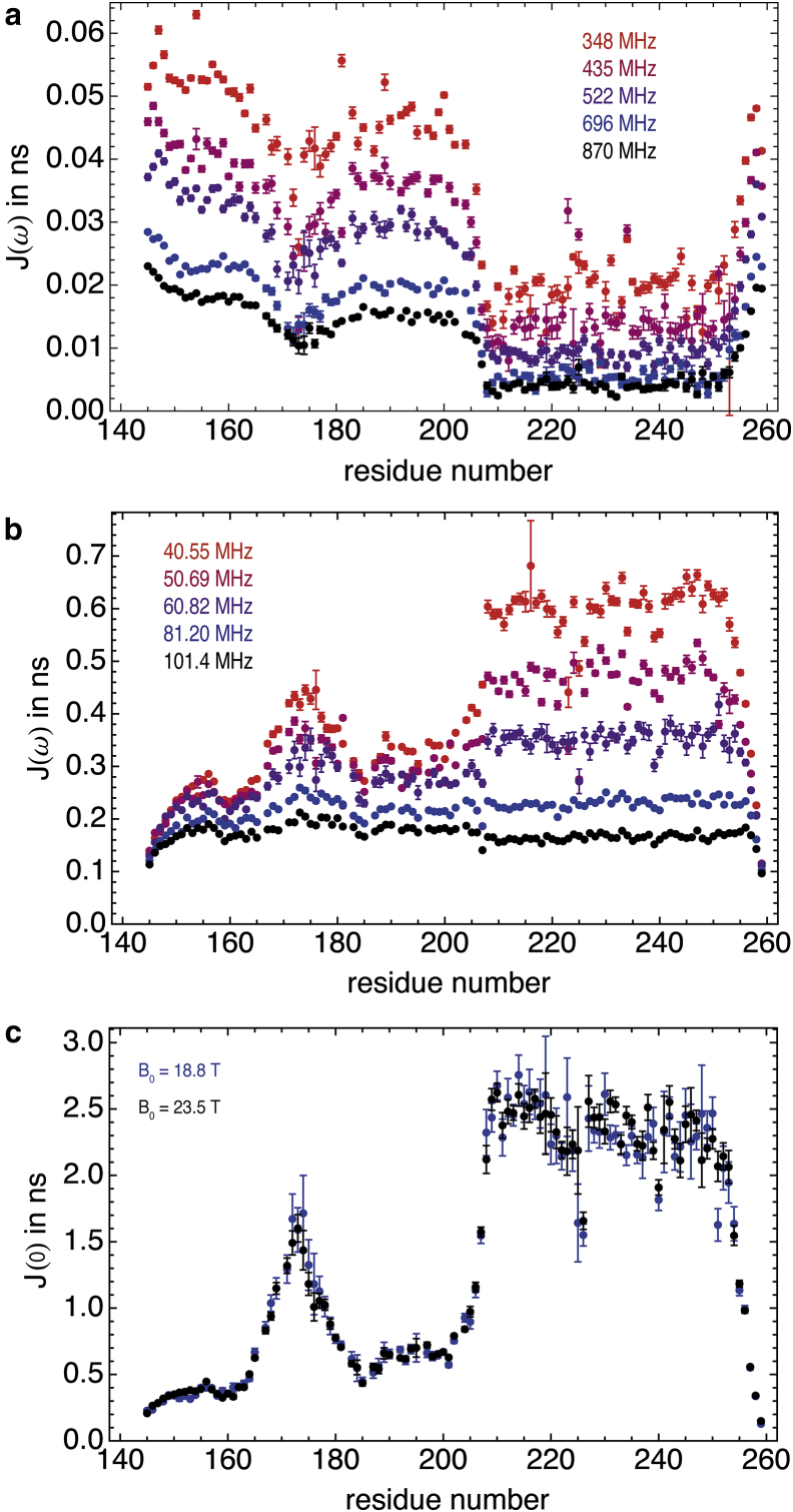
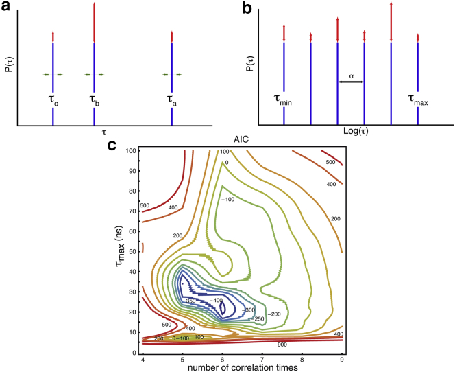
Intrinsically disordered proteins and intrinsically disordered regions (IDRs) are ubiquitous in the eukaryotic proteome. The description and understanding of their conformational properties require the development of new experimental, computational, and theoretical approaches. Here, we use nuclear spin relaxation to investigate the distribution of timescales of motions in an IDR from picoseconds to nanoseconds. Nitrogen-15 relaxation rates have been measured at five magnetic fields, ranging from 9.4 to 23.5 T (400-1000 MHz for protons). This exceptional wealth of data allowed us to map the spectral density function for the motions of backbone NH pairs in the partially disordered transcription factor Engrailed at 11 different frequencies. We introduce an approach called interpretation of motions by a projection onto an array of correlation times (IMPACT), which focuses on an array of six correlation times with intervals that are equidistant on a logarithmic scale between 21 ps and 21 ns. The distribution of motions in Engrailed varies smoothly along the protein sequence and is multimodal for most residues, with a prevalence of motions around 1 ns in the IDR. We show that IMPACT often provides better quantitative agreement with experimental data than conventional model-free or extended model-free analyses with two or three correlation times. We introduce a graphical representation that offers a convenient platform for a qualitative discussion of dynamics. Even when relaxation data are only acquired at three magnetic fields that are readily accessible, the IMPACT analysis gives a satisfactory characterization of spectral density functions, thus opening the way to a broad use of this approach.

Figure 1

Backbone ¹⁵N relaxation rates and NOEs measured in Engrailed 2 at five magnetic fields: 400 MHz (red), 500 MHz (burgundy), 600 MHz (purple), 800 MHz (blue), and 1000 MHz (black). (a) Longitudinal relaxation rates, R₁, of ¹⁵N. (b) ¹⁵N-{¹H} NOE ratios. (c) Longitudinal cross-relaxation rates, η_z, due to correlated fluctuations of the ¹⁵N CSA and the ¹⁵N-¹H dipolar couplings. (d) Transverse cross-relaxation rates, η_xy, due to the same correlated fluctuations. (e) SSP calculated from the chemical shifts of carbonyl and α and β carbon-13 nuclei. To see this figure in color, go online.

Figure 2

Spectral density functions for backbone NH vectors in Engrailed 2. (a) Effective spectral density near the proton Larmor frequency, J(0.87ω_H) (ns). (b) Spectral density at the Larmor frequency of nitrogen-15, J(ω_N) (ns). (c) Spectral density at zero frequency, J(0) (ns). All data are color-coded as a function of the magnetic field at which the relaxation rates were recorded, with the same code as in Fig. 1. To see this figure in color, go online.

Figure 3

Principle and optimization of the parameters of our IMPACT analysis. (a) In the 3CT analysis, both the value and the relative weight of each correlation time must be adjusted. (b) In IMPACT, the values of the correlation times are fixed and equally spaced on a logarithmic scale, so that only their relative weights need adjusting. (c) Optimization of IMPACT by considering AIC. The range (τ_min, τ_max) of correlation times characterized by IMPACT was varied from (1 ps, 1 ns) to (100 ps, 100 ns) and the number of correlation times was varied in the range n = 4–9. Despite the solid lines shown in the contour plot (c), the reader should be aware that the number of correlation times is an integer. To see this figure in color, go online.

Figure 4

Plots of the six coefficients, A_i (i = 1, 2… 6) of the n = 6 correlation times, τ_i, in the range [τ_min, τ_max] = [21 ps, 21 ns] determined by the IMPACT analysis of Engrailed: (a) τ₁ = 21 ns; (b) τ₂ = 5.27 ns; (c) τ₃ = 1.33 ns; (d) τ₄ = 333 ps; (e) τ₅ = 83.6 ps; (f) τ₆ = 21 ps. To see this figure in color, go online.

Figure 5

Graphical representations of (a) IMPACT, (c) 2CT, and (d) 3CT analyses of the spectral density function in Engrailed 2. Histograms are drawn for all residues and represent the contributions of (a) each of the six correlation times, τ_i (i = 1, 2, …6), considered in IMPACT, (c) each of the two correlation times, τ_a,b, determined by the 2CT analysis, (d) each of the three correlation times, τ_a,b,c, determined by the 3CT analysis. The width of each rectangle is proportional to the corresponding weights A_i in IMPACT (a), B_a,b in 2CT (c); and B_a,b,c in 3CT (d). In (c) and (d), the light blue horizontal bars represent the ranges of correlation times, τ, for which reciprocal frequencies lie in the constrained regions between 40 < 1/(2π τ) < 100 MHz or between 348 < 1/(2πτ) < 870 MHz. Gray rectangles in (a), (c), and (d) indicate rigid α-helices, and a green rectangle shows the rigid hydrophobic hexapeptide sequence. (b) As in Fig. 1e, the SSP is shown to guide the comparison between structural and dynamic features. To see this figure in color, go online.

Figure 6

Results obtained for a conventional analysis with 2CT (blue) or 3CT (red). (a) Order parameter S². (b) Order parameter S²_f for the fastest motion in the 3CT analysis. (c) Longest correlation time, τ_a. (d and e) Intermediate correlation time, τ_b (d), and shortest correlation time, τ_c (e). Either the 2CT or the 3CT model was selected based on the lowest AIC. To see this figure in color, go online.

References

1. van der Lee R., Buljan M., Babu M.M. Classification of intrinsically disordered regions and proteins. Chem. Rev. 2014;114:6589–6631. - PMC - PubMed
1. Dyson H.J., Wright P.E. Intrinsically unstructured proteins and their functions. Nat. Rev. Mol. Cell Biol. 2005;6:197–208. - PubMed
1. Uversky V.N., Dunker A.K. Understanding protein non-folding. Biochim. Biophys. Acta. 2010;1804:1231–1264. - PMC - PubMed
1. Dunker A.K., Lawson J.D., Obradovic Z. Intrinsically disordered protein. J. Mol. Graph. Model. 2001;19:26–59. - PubMed
1. Jensen M.R., Markwick P.R.L., Blackledge M. Quantitative determination of the conformational properties of partially folded and intrinsically disordered proteins using NMR dipolar couplings. Structure. 2009;17:1169–1185. - PubMed
Publication types