. 2015 Oct;33(10):1045-52.
doi: 10.1038/nbt.3319. Epub 2015 Sep 7.

ConStrains identifies microbial strains in metagenomic datasets

Affiliations

ConStrains identifies microbial strains in metagenomic datasets

Chengwei Luo et al. Nat Biotechnol. 2015 Oct.

Abstract

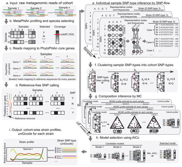
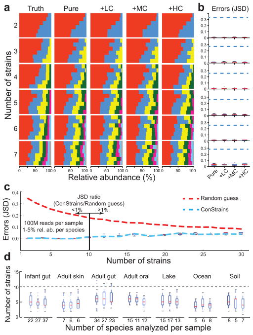
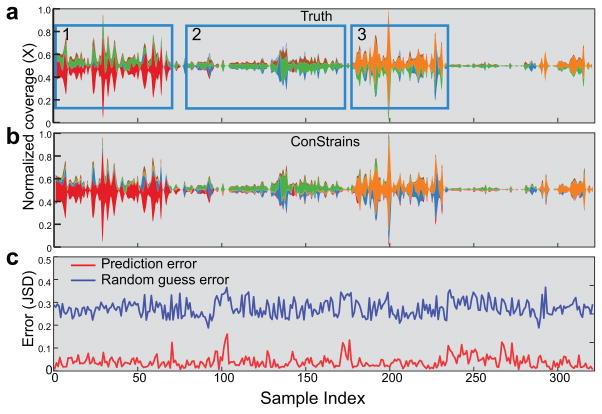
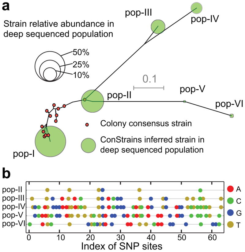
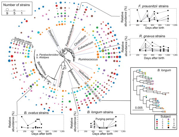
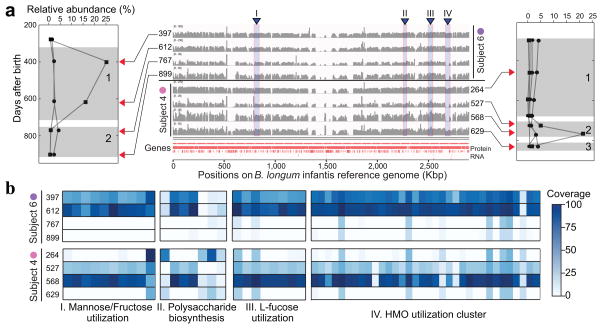
An important fraction of microbial diversity is harbored in strain individuality, so identification of conspecific bacterial strains is imperative for improved understanding of microbial community functions. Limitations in bioinformatics and sequencing technologies have to date precluded strain identification owing to difficulties in phasing short reads to faithfully recover the original strain-level genotypes, which have highly similar sequences. We present ConStrains, an open-source algorithm that identifies conspecific strains from metagenomic sequence data and reconstructs the phylogeny of these strains in microbial communities. The algorithm uses single-nucleotide polymorphism (SNP) patterns in a set of universal genes to infer within-species structures that represent strains. Applying ConStrains to simulated and host-derived datasets provides insights into microbial community dynamics.


Conflict of interest statement

Competing Financial Interests

The authors declare no competing financial interests.

Figures

Figure 1
Figure 1
Overview of the ConStrains algorithm: from raw metagenomic data to strain profiles and uniGcodes. (a) ConStrains requires raw metagenomic reads from a single or series of metagenomic samples as input. (b) To select species that satisfy a predefined sequencing depth cutoff, the algorithm starts with determining the species composition with MetaPhlAn. (c) Next, Bowtie2 is used to recruit all reads to a reference database of species-specific marker genes. (d) SNPs are called on these recruited reads after quality filtering, removal of reference gene sequence, and reference-free read realignment. (e) Resulting SNPs are used by a SNP-flow algorithm to infer all possible SNP-types for each of the samples. (f) Such SNP-types across samples are clustered using a tree structure based on their distances to represent candidate strain models; the internal distance cutoff, Δd, is varied to exhaust all possible SNP-type clusterings. (g) The Metropolis-Hastings Monte-Carlo method is then carried out to infer relative abundances per sample and per species for every candidate strain model. (h) These models are then evaluated by corrected Akaike information criterion (AICc) and the model with minimum AICc is selected as the optimal model. (i) Finally, the associated strains’ relative abundances across samples and their uniGcodes are generated for every species.
Figure 2
Figure 2. ConStrains correctly predicts the strain composition of in silico-simulated data sets
A comparison of true and predicted strain composition profiles of in silico-simulated multi-strain mixtures is shown. (a) An increasing number of multi-strain mixtures (n = 2–7; rows) was analyzed with ConStrains either containing only the target strains (pure) or in the context of a metagenome of low, medium, and high complexity (+LC, +MC, and +HC, respectively). In each box of barcharts, the colors represent different strains that were mixed in six different ratios (x axis, relative abundance) with a Shannon index (y axis) increasing from top to bottom. In the resulting 144 admixtures, all strains were correctly identified. (b) To compare the predictions in abundance for each strain, the Jensen-Shannon Divergence (JSD) between predicted composition and the true composition was determined. Blue dashed lines mark the expected errors from random guesses. The box marks the interquartile range, the red bar marks the interquartile median, whiskers represent the top and the bottom 25% data range, and outliers are marked by crosses. Good performance was obtained for all compositions, with minimal difference in the accuracy of results between pure mixtures and metagenomic mixtures; see also Supplementary Fig. 3b for more detailed graphs. (c) Graph showing ConStrains’ ability to correctly infer intra-specific structure as a function of the number of strains contained in a sample. Shown is a typical case with the species’ relative abundance ranging from 1% to 5% and a sequencing depth of 100 million paired-end reads, though higher abundance or sequencing depth would improve its accuracy. The ConStrains’ prediction JSD errors (blue dashed line and boxes) were below 1% of null informative prediction errors (random guess; red dashed line) when the number of strains within a species was less than ten. (d) For comparison, three metagenomic samples were randomly chosen from seven different niches, ranging from adult gut microbiome to a marine planktonic community. More than 95% of the species from these metagenomic samples possessed fewer than ten strains (dashed horizontal line). Dashed lines and whiskers mark the interquartile range; plusses mark the outliers.
Figure 3
Figure 3
ConStrains scales to large time series and accurately predicts strain dynamics. In the absence of existing large time series metagenomic data sets, a simulated set with 322 samples was created. Shown are the strain predictions within the Bacteroides fragilis species. The (a) true and (b) ConStrains-predicted relative abundance (y axis) of B. fragilis strains (stream ribbon width, with different colors representing different strains) in different samples sorted in longitudinal order (x axis, sample index) are illustrated. Inset windows 1–3 in a indicate periods with different dominant strains. (c) Prediction errors (red line) in each sample were measured between the true and predicted profiles using Jenson-Shannon Divergence (y axis, JSD). For comparison, random guess error (blue line) is shown to indicate a lower performance boundary. Spikes in error rates above 0.1 JSD are mostly related to time points in which the species average coverage drops below 10×, preventing reliable SNP profiling (Supplementary Fig. 7b).
Figure 4
Figure 4. High sensitivity identification of strain phylogeny within a cystic fibrosis Burkholderia dolosa population data set
ConStrains was used to re-analyze data from a published study on the genetic variation of Burkholderia dolosa populations within cystic fibrosis patients. (a) A total of six B. dolosa strains (pop-I to pop-VI) were predicted with an abundance of > 0.1% of the species (diameter of green circles proportional to relative abundance). An unrooted neighbor-joining tree on the alignments of the unweighted concatenated SNP profiles was constructed for the predicted strains (green circles) and the corresponding genomic data for the 29 cultured isolates (red circles; gray bar indicates the tree distance scale). These results show that the original study retrieved numerous isolates for the two most dominant strains within the population, but could not isolate the lower abundance strains. Distance between predicted strains and isolates fall within the prediction sensitivity of the ConStrains algorithm (same strain individuals differ with no more than 5% of all SNPs). (b) To demonstrate the sensitivity of the algorithm for differentiating strains, the color-coded allelic difference for each of the predicted strains is shown in reference to the most dominant strain, pop-I. Sites with the same allele as reference (pop-I) were not marked.
Figure 5
Figure 5
ConStrains analysis reveals species longitudinal dynamics and functional shifts within an infant gut development cohort. A cohort of nine infants that were sampled throughout the first three years of life, and for which metagenomic data was available for up to nine time points, were analyzed with ConStrains. For a total of 75 species, the depth was sufficient to interpret the underlying strains. The circular tree is constructed using a representative sequence for each species, with the colored outer rings indicating the number of strains observed for each of the nine subjects. Open boxes show the longitudinal dynamics of strains in four selected species; the phylogeny tree insert box shows all strains including the available reference genome of B. longum.
Figure 6
Figure 6. Functional differences in Bifidobacterium longum strains at different time points during infant gut microbiome development
(a) Two subjects experienced dominant strain switches within the species B. longum (flanking panels, periods marked by numbered gray shadows). Each track in the middle panel shows the corresponding sample’s coverage over the B. longum reference genome. Time points (days after birth) are marked by red triangles. Windows I–IV capture gene content differences before and after dominant strain switches, reflected by the reference genome. (b) The four highlighted regions (I–IV in a) indicate strain-specific functional cohesion that is also strongly associated with B. longum relative abundance in gut microbiome development.

References

    1. Segata N, et al. Metagenomic microbial community profiling using unique clade-specific marker genes. Nat Methods. 2012;9:811–814. - PMC - PubMed
    1. Sunagawa S, et al. Metagenomic species profiling using universal phylogenetic marker genes. Nat Methods. 2013;10:1196–1199. - PubMed
    1. Darling AE, et al. PhyloSift: phylogenetic analysis of genomes and metagenomes. PeerJ. 2014;2:e243. - PMC - PubMed
    1. Sharon I, et al. Time series community genomics analysis reveals rapid shifts in bacterial species, strains, and phage during infant gut colonization. Genome Res. 2013;23:111–120. - PMC - PubMed
    1. Nielsen HB, et al. Identification and assembly of genomes and genetic elements in complex metagenomic samples without using reference genomes. Nat Biotechnol. 2014;32:822–828. - PubMed

Publication types