An automated sleep-state classification algorithm for quantifying sleep timing and sleep-dependent dynamics of electroencephalographic and cerebral metabolic parameters

Abstract

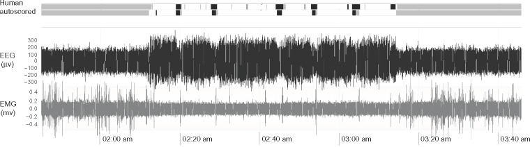
Introduction: Rodent sleep research uses electroencephalography (EEG) and electromyography (EMG) to determine the sleep state of an animal at any given time. EEG and EMG signals, typically sampled at >100 Hz, are segmented arbitrarily into epochs of equal duration (usually 2-10 seconds), and each epoch is scored as wake, slow-wave sleep (SWS), or rapid-eye-movement sleep (REMS), on the basis of visual inspection. Automated state scoring can minimize the burden associated with state and thereby facilitate the use of shorter epoch durations.

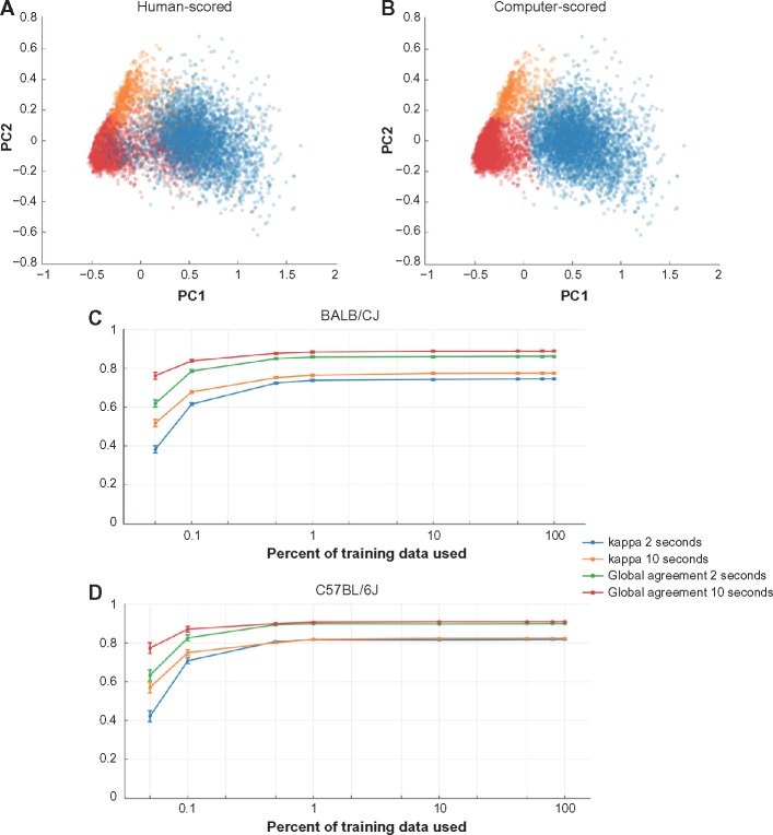
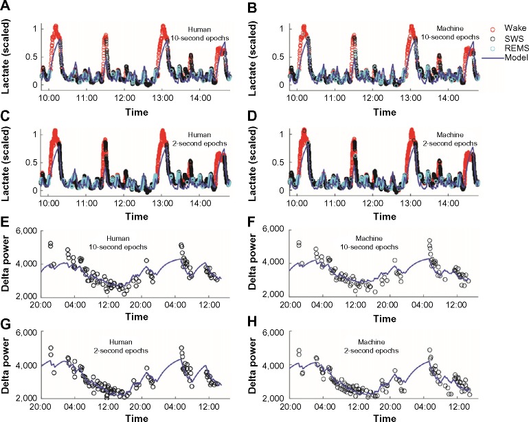
Methods: We developed a semiautomated state-scoring procedure that uses a combination of principal component analysis and naïve Bayes classification, with the EEG and EMG as inputs. We validated this algorithm against human-scored sleep-state scoring of data from C57BL/6J and BALB/CJ mice. We then applied a general homeostatic model to characterize the state-dependent dynamics of sleep slow-wave activity and cerebral glycolytic flux, measured as lactate concentration.

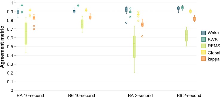
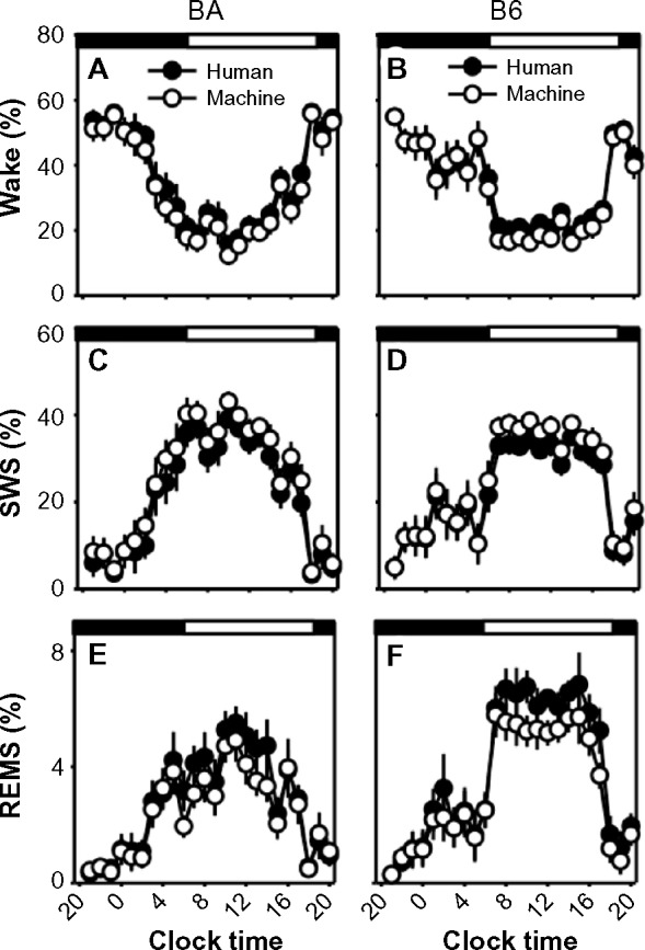
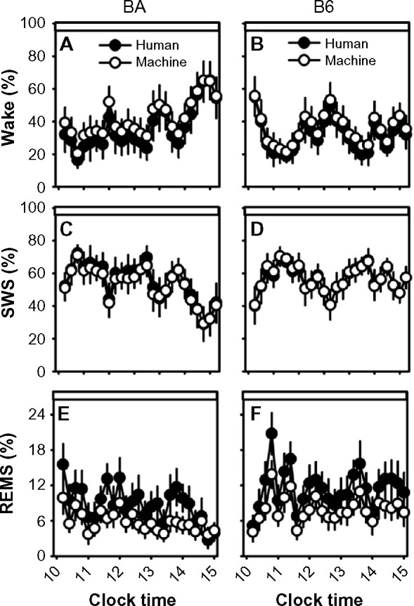
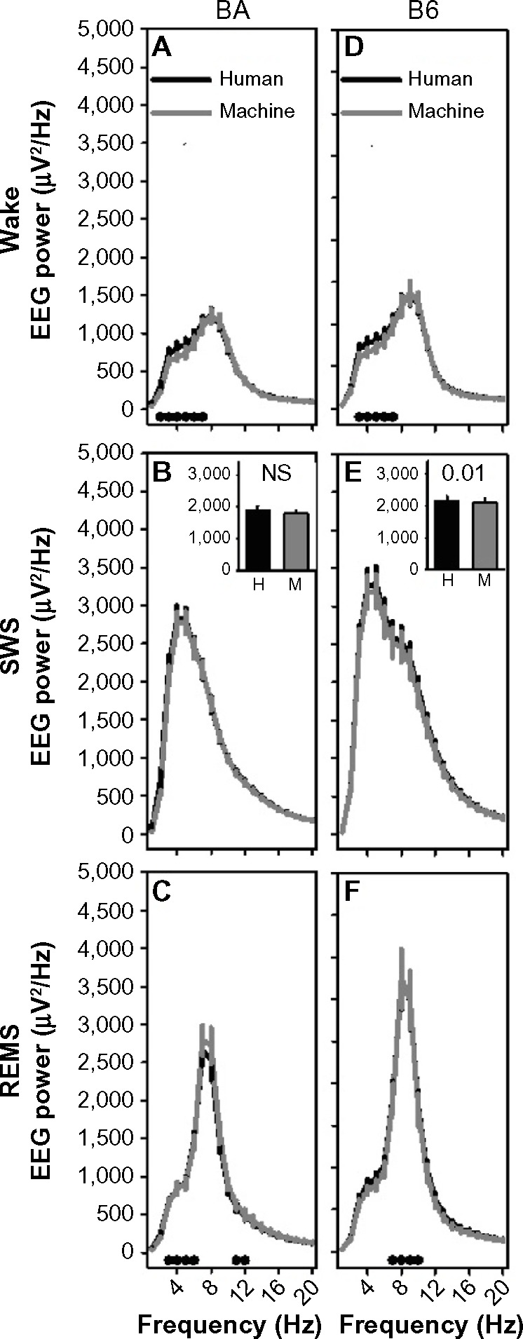
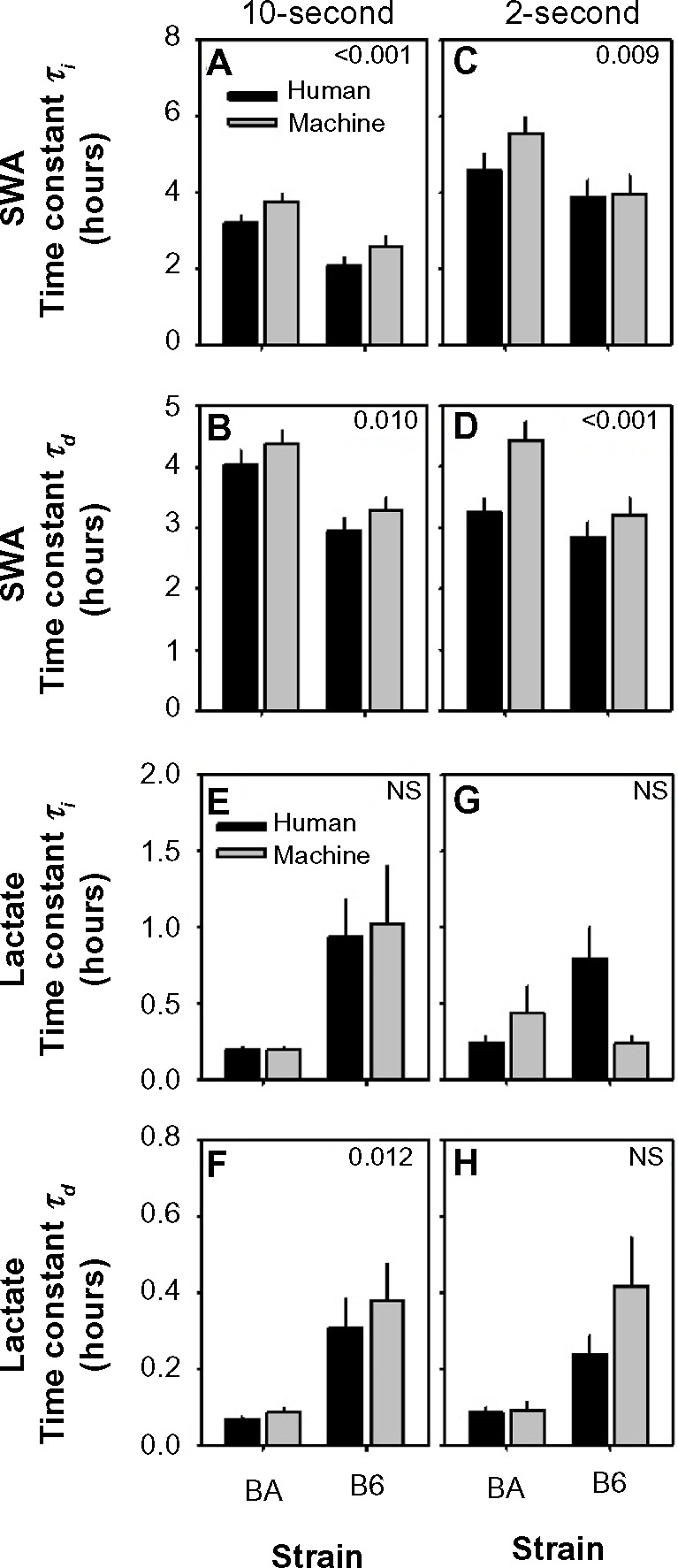
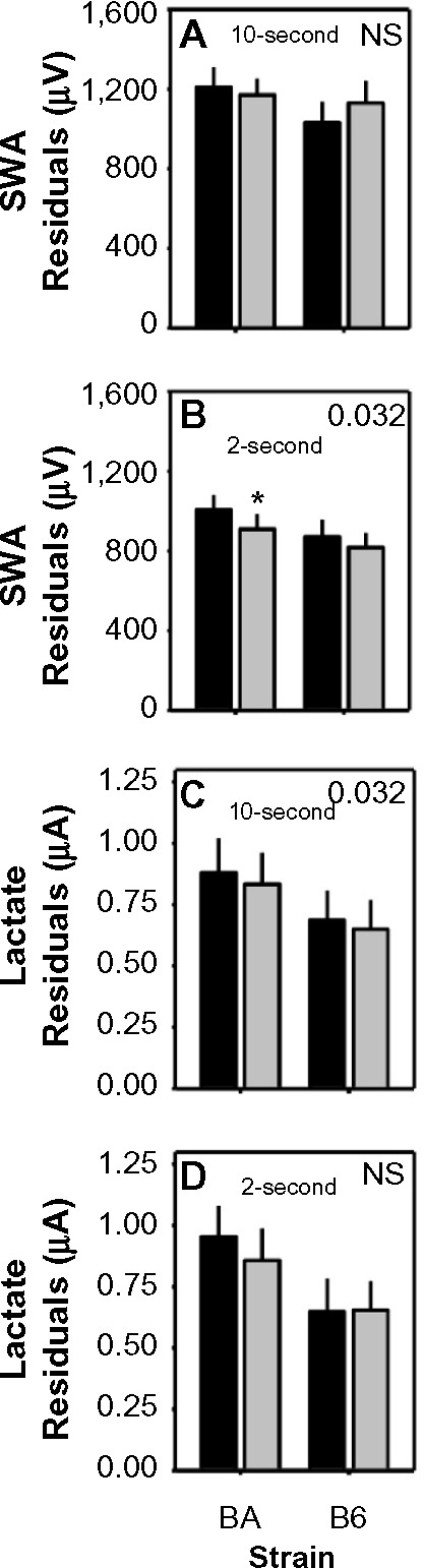
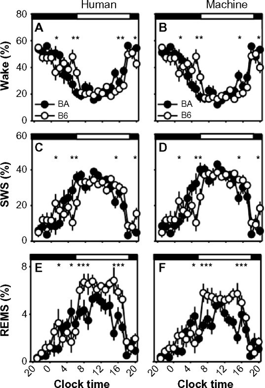
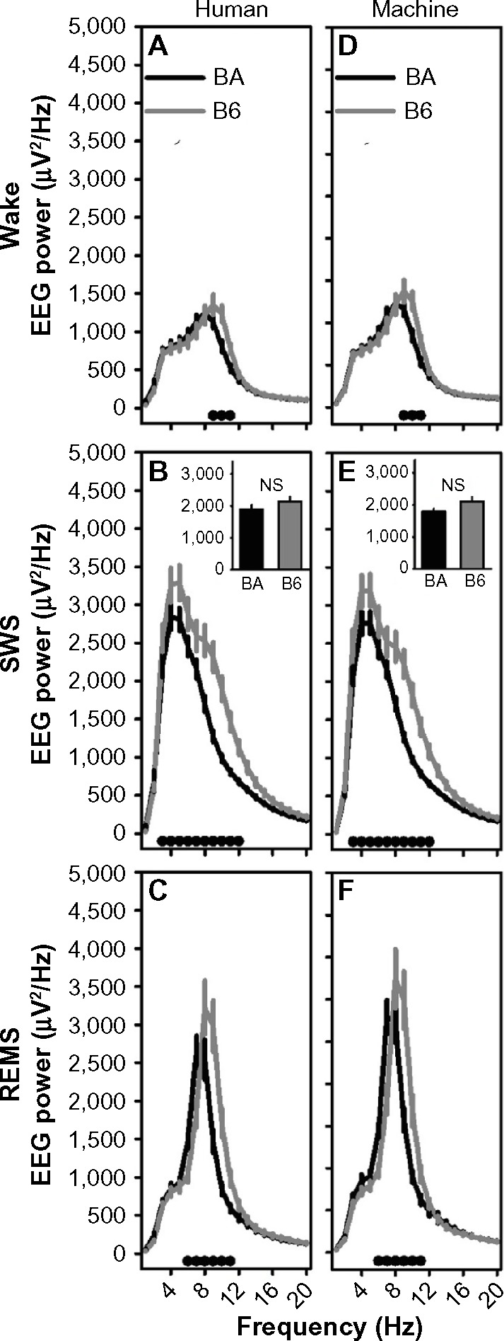
Results: More than 89% of epochs scored as wake or SWS by the human were scored as the same state by the machine, whether scoring in 2-second or 10-second epochs. The majority of epochs scored as REMS by the human were also scored as REMS by the machine. However, of epochs scored as REMS by the human, more than 10% were scored as SWS by the machine and 18 (10-second epochs) to 28% (2-second epochs) were scored as wake. These biases were not strain-specific, as strain differences in sleep-state timing relative to the light/dark cycle, EEG power spectral profiles, and the homeostatic dynamics of both slow waves and lactate were detected equally effectively with the automated method or the manual scoring method. Error associated with mathematical modeling of temporal dynamics of both EEG slow-wave activity and cerebral lactate either did not differ significantly when state scoring was done with automated versus visual scoring, or was reduced with automated state scoring relative to manual classification.

Conclusions: Machine scoring is as effective as human scoring in detecting experimental effects in rodent sleep studies. Automated scoring is an efficient alternative to visual inspection in studies of strain differences in sleep and the temporal dynamics of sleep-related physiological parameters.

Keywords: Bayes classification; EEG; automated scoring; principal component analysis.

Figure 1

Comparison of human scoring to machine scoring. Notes: Principal component plots of a 43-hour recording scored in 10-second epochs by a human (A) and using the machine learning algorithm (B). Each dot represents one 10-second epoch, and its color represents sleep state (SWS = blue, wake = red, REMS = orange). The computer-scored plot used data from 10 am to 2 pm (Zeitgeber time 4–8 in the first complete light/dark cycle of the recording) as training data to score every epoch in the entire 43-hour recording. Both for BALB/CJ mice (C) and C57BL/6J mice (D), the agreement between machine-scored and human-scored increased as more of the training data were used. For each genetic strain, 8,640 2-second epochs and 8,640 10-second epochs were scored by a human and by the autoscoring procedure, with 0.05%, 0.1%, 0.5%, 1%, 10%, 50%, 80%, and 100% of those 8,640 epochs used as training data. These correspond to 4 epochs, 9 epochs, 43 epochs, 86 epochs, 864 epochs, 4,320 epochs, 6,912 epochs, and 8,640 epochs, respectively. In each case it was ensured that at least one epoch of each state was present. Two measures of agreement between the human scoring and the machine scoring were computed: Cohen’s kappa and global agreement. The x-axis shows the percentage of the 8,640 epochs used as training data, indicating that the learning algorithm requires only about 1% of the training data to reach optimal performance. Abbreviations: REMS, rapid-eye-movement sleep; SWS, slow-wave sleep.

Figure 2

EEG and EMG data for comparison of human scoring and machine scoring. Notes: The top two traces show human and autoscored sleep states for each 10-second epoch of the EEG and EMG shown in the lower panels. The sleep states are labeled with color (gray for wake, white for SWS, and black for REMS). Abbreviations: EEG, electroencephalography; EMG, electromyography; REMS, rapid-eye-movement sleep; SWS, slow-wave sleep.

Figure 3

Agreement statistics between human scoring and machine scoring. Notes: For the data scored in 10-second epochs, the agreement statistics compare the human and machine scoring for the entire 40–48-hour recording. For the data in 2-second epochs, the comparison is between 8,640 epochs that were scored by hand and the same 8,640 epochs scored by the automated scoring algorithm. Lines inside boxes represent median values. The lower end of each box indicates the first quartile of the data (Q1), and the upper end represents the third quartile (Q3). To draw the whiskers, we calculated the interquartile range (IQR), which is the distance between Q1 and Q3. The lower whisker indicates the lowest data point within 1.5 IQR of Q1. The upper whisker indicates the largest data point within 1.5 IQR of Q3. Outliers more than 1.5 IQR but less than 3 IQR above Q3 or below Q1 are represented with open circles. Abbreviations: B6, C57BL/6J mice; BA, BALB/CJ mice; REMS, rapid-eye-movement sleep; SWS, slow-wave sleep.

Figure 4

Sleep-state percentages in human-scored versus machine-scored 10-second epoch data. Notes: Data from the BA strain (left column) and the B6 strain (right column), were binned into 60-minute intervals. Graphs represent the percentage of each interval spent in wake (A and B), SWS (C and D), and REMS (E and F). Open circles represent machine-scored data and filled circles represent human-scored data. Dark and light phases are indicated by black and white bands at the top of each panel. Abbreviations: B6, C57BL/6J mice; BA, BALB/CJ mice; REMS, rapid-eye-movement sleep; SWS, slow-wave sleep.

Figure 5

Sleep-state percentages in human-scored versus machine-scored 2-second epoch data. Notes: Data from the BA strain (left column) and the B6 strain (right column) were binned into 12-minute intervals. Graphs represent the percentage of each interval spent in wake (A and B), SWS (C and D), and REMS (E and F). Open circles represent machine-scored data and filled circles represent human-scored data. Data are from Zeitgeber time 4–9. Abbreviations: B6, C57BL/6J mice; BA, BALB/CJ mice; REMS, rapid-eye-movement sleep; SWS, slow-wave sleep.

Figure 6

Machine-scored data in 10-second epochs exhibit similar frequency profiles to human-scored data. Notes: The left column shows data for the BA strain and the right column shows data for the B6 strain. For wake (A and D), SWS (B and E), and REMS (C and F), the frequency profiles of the human-scored data (black line) and those of the machine-scored data (gray line) are shown. The black dots in panels (A, C, D and F) indicate frequency bands in which posthoc comparisons (Fisher’s protected least-significant difference) indicated a difference between the curves. The insets in panels (B and E) show 1–4 Hz SWA. P-values in these insets indicate main effect of scoring method on SWA. Abbreviations: B6, C57BL/6J mice; BA, BALB/CJ mice; EEG, electroencephalography; EMG, electromyography; H, human; M, machine; NS, not significant; REMS, rapid-eye-movement sleep; SWA, slow-wave activity; SWS, slow-wave sleep.

Figure 7

Homeostatic modeling of lactate data and SWA scored by human or machine. Notes: The left column shows human-scored data and the right-hand column shows machine-scored data. The top four panels show scaled lactate data in 10-second epochs scored by a human (A), 10-second epochs autoscored (B), 2-second epochs scored by a human (C), and 2-second epochs autoscored (D). The bottom four panels show SWA in 5-minute sleep episodes using 10-second epochs scored by a human (E), 10-second epochs autoscored (F), 2-second epochs scored by a human (G), and 2-second epochs autoscored (H). In each panel, a homeostatic model for lactate or SWA was fit to the data (solid curve). The difference in time scale between the lower panels and the upper panels reflects the difference in temporal dynamics of SWA versus those of lactate. Abbreviations: REMS, rapid-eye-movement sleep; SWA, slow-wave activity; SWS, slow-wave sleep.

Figure 8

Strain differences in optimal time constants in general homeostatic modeling of state-dependent SWA and lactate dynamics. Notes: Data represent optimized time constants for wake/REMS-dependent increases (τ_i) and SWS-dependent decreases (τ_d) in SWA (A–D) and lactate (E–H) from human-scored data (black bars) and machine-scored data (gray bars). P-values are shown for main effect of scoring method on time constants. Abbreviations: B6, C57BL/6J mice; BA, BALB/CJ mice; NS, not significant; REMS, rapid-eye-movement sleep; SWA, slow-wave activity; SWS, slow-wave sleep.

Figure 9

Differences in residuals of model fit to data scored by human or machine. Notes: Data represent the residuals associated with optimized time constants for modeling SWA (A and B) and lactate (C and D) from human-scored data (black bars) and machine-scored data (gray bars) in either 10-second or 2-second epochs. P-values are shown for main effect of scoring method on time constants. Asterisk denotes significant difference for human versus machine scoring within the BA strain (Fisher’s protected least-significant difference). Abbreviations: B6, C57BL/6J mice; BA, BALB/CJ mice; NS, not significant; R SWA, slow-wave activity.

Figure 10

Strain differences in sleep/wake state timing scored in 10-second epochs. Notes: Strain differences in the time course of sleep/wake states were observed in human-scored data (A, C and E) or machine-scored data (B, D and F). Filled circles represent data from the BA strain, and open circles represent data from the B6 strain. Asterisks indicate 60-minute epochs in which there is a statistically significant difference between strains (Fisher’s protected least-significant difference). Timing of the dark and light phases of the 12:12 cycle is indicated by the black and white bars at the top of each graph. Abbreviations: B6, C57BL/6J mice; BA, BALB/CJ mice; REMS, rapid-eye-movement sleep; SWS, slow-wave sleep.

Figure 11

Strain differences in EEG power spectra in 10-second epochs scored by human or machine. Notes: The left column shows human-scored data and the right column shows machine-scored data. For wake (A and D), SWS (B and E), and REMS (C and F), EEG power differed between strains at specific frequencies. The black dots at the base of each graph indicate frequency bands in which posthoc comparisons (Fisher’s protected least-significant difference) indicated a difference between the BA (black line) and B6 (gray line) strains. The insets in panels (B and (E) show 1–4 Hz SWA, which did not differ between strains. Abbreviations: B6, C57BL/6J mice; BA, BALB/CJ mice; EEG, electroencephalography; NS, not significant; REMS, rapid-eye-movement sleep; SWS, slow-wave sleep.

References

1. Stephenson R, Caron AM, Cassel DB, Kostela JC. Automated analysis of sleep-wake state in rats. J Neurosci Methods. 2009;184(2):263–274. - PubMed
1. Gilmour TP, Fang J, Guan Z, Subramanian T. Manual rat sleep classification in principal component space. Neurosci Lett. 2010;469(1):97–101. - PMC - PubMed
1. Rytkönen KM, Zitting J, Porkka-Heiskanen T. Automated sleep scoring in rats and mice using the naive Bayes classifier. J Neurosci Methods. 2011;202(1):60–64. - PubMed
1. Brankack J, Kukushka VI, Vyssotski AL, Draguhn A. EEG gamma frequency and sleep-wake scoring in mice: comparing two types of supervised classifiers. Brain Res. 2010;1322:59–71. - PubMed
1. Gross BA, Walsh CM, Turakhia AA, Booth V, Mashour GA, Poe GR. Open-source logic-based automated sleep scoring software using electrophysiological recordings in rats. J Neurosci Methods. 2009;184(1):10–18. - PMC - PubMed
LinkOut - more resources