Prospective Optimization with Limited Resources

Abstract

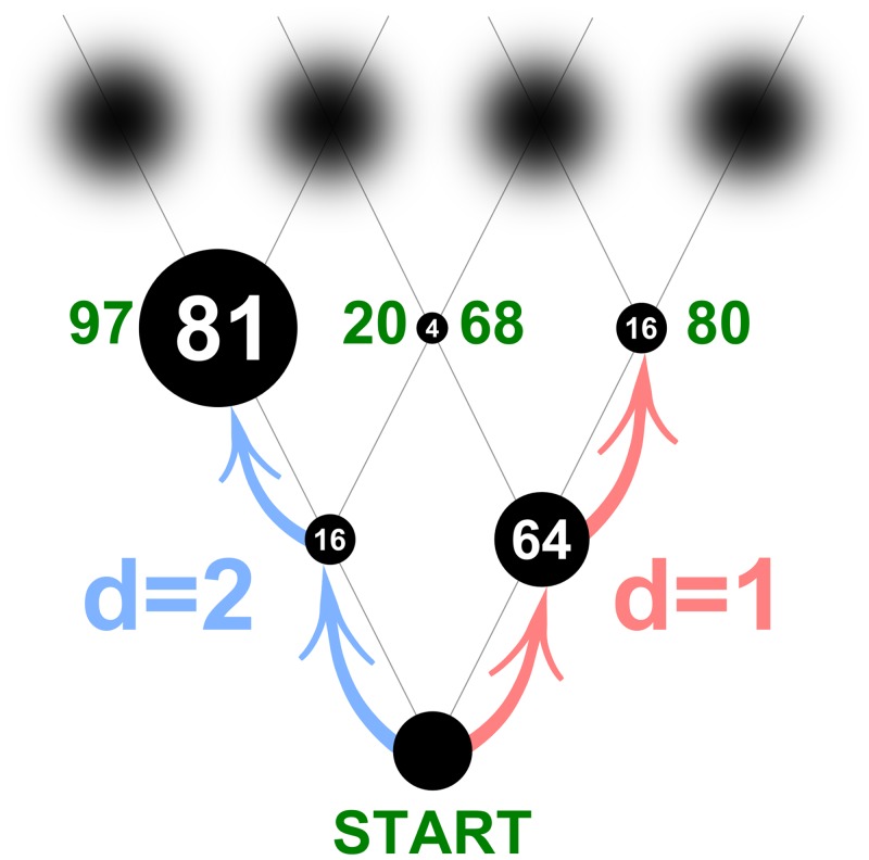
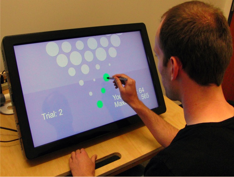
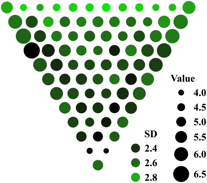
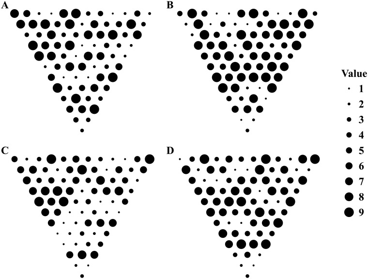
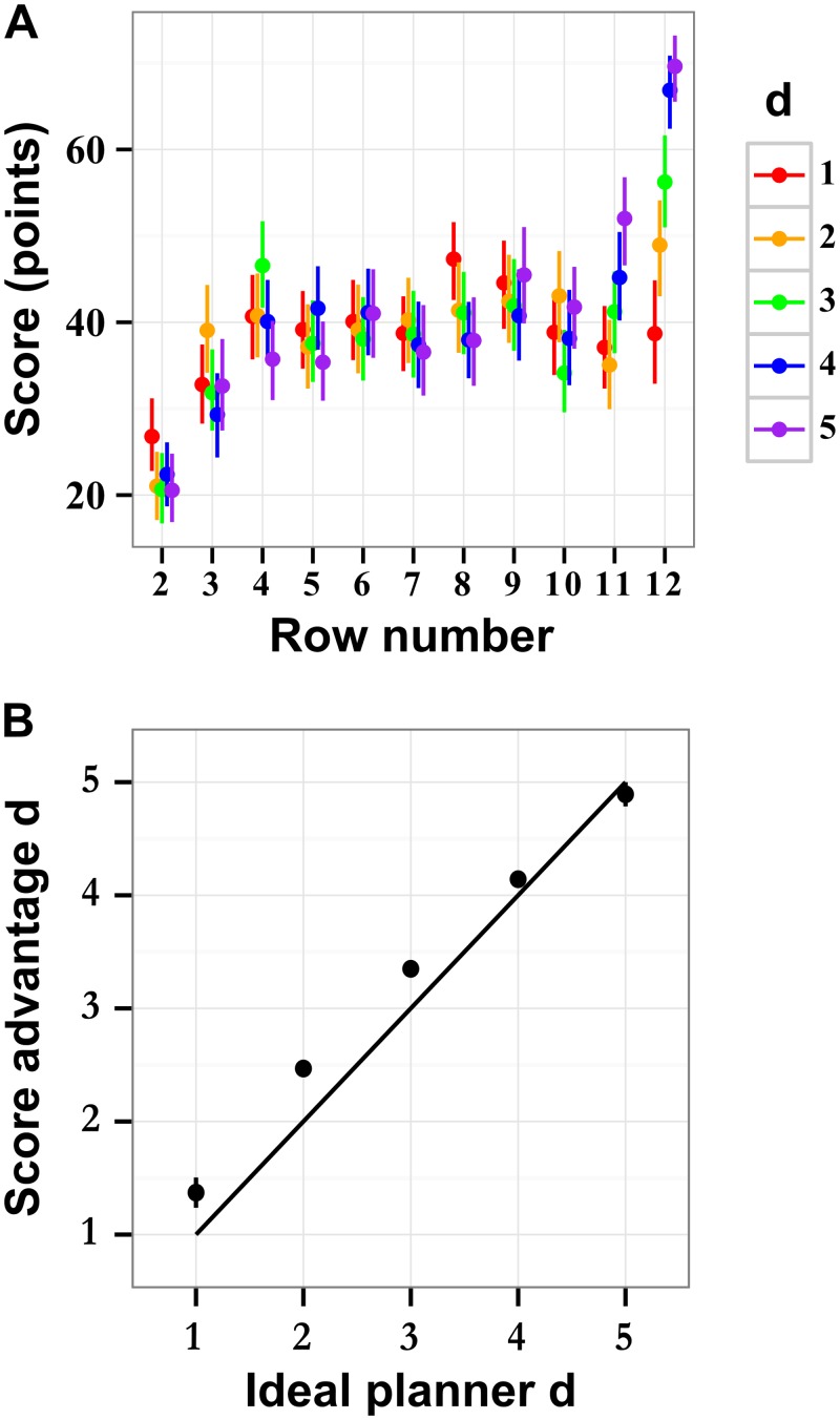
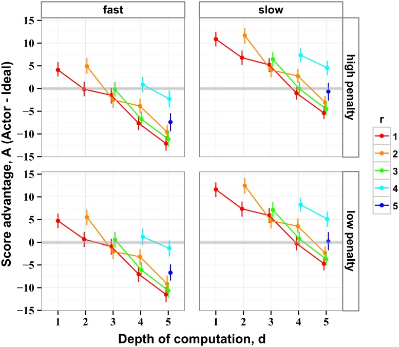
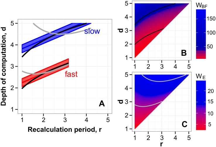
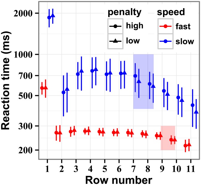
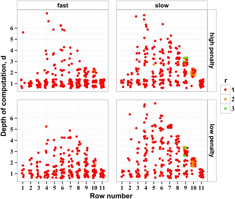
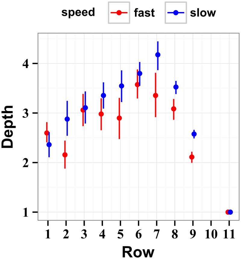
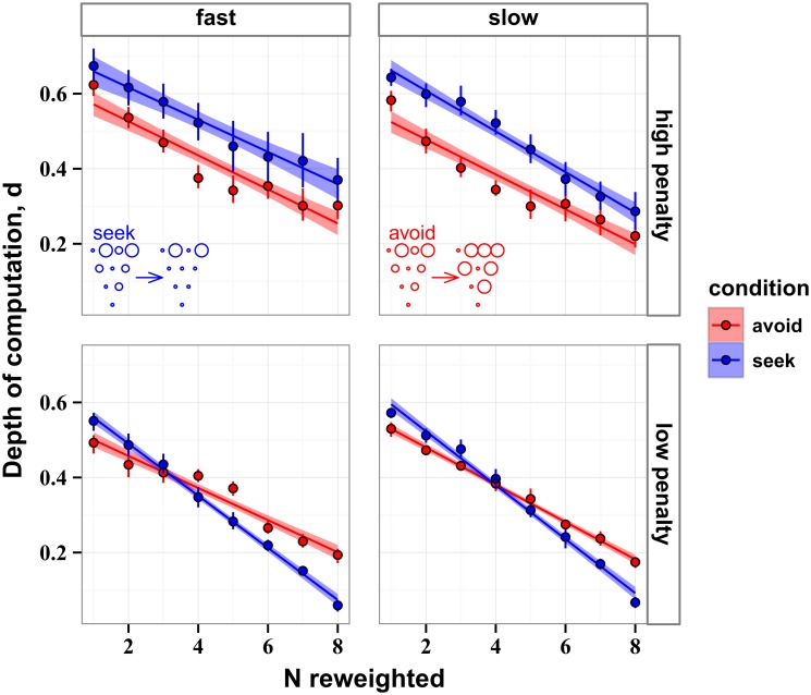
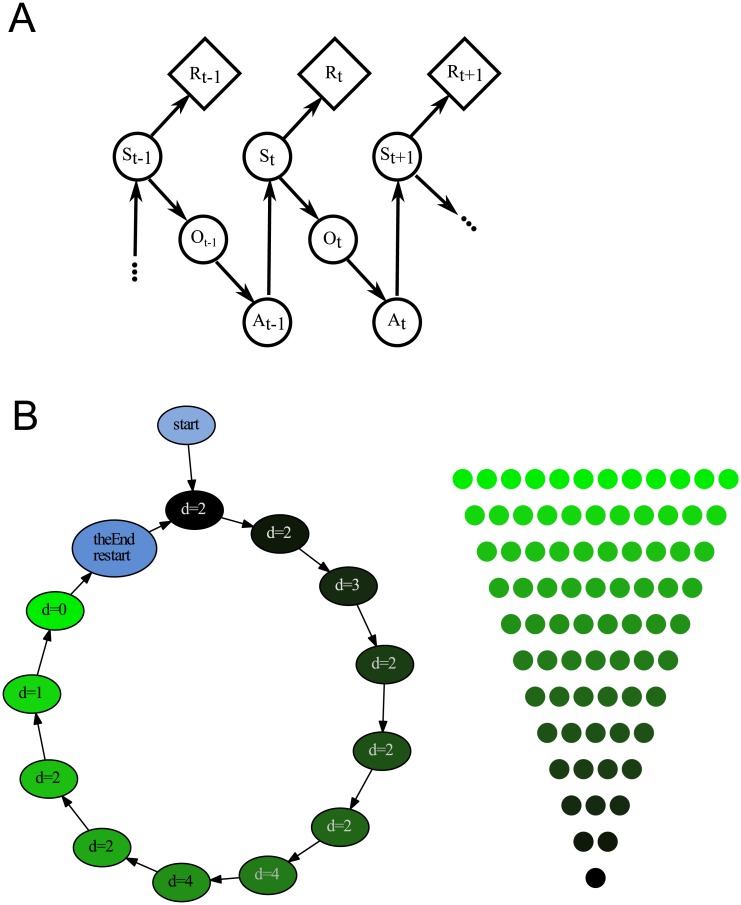
The future is uncertain because some forthcoming events are unpredictable and also because our ability to foresee the myriad consequences of our own actions is limited. Here we studied how humans select actions under such extrinsic and intrinsic uncertainty, in view of an exponentially expanding number of prospects on a branching multivalued visual stimulus. A triangular grid of disks of different sizes scrolled down a touchscreen at a variable speed. The larger disks represented larger rewards. The task was to maximize the cumulative reward by touching one disk at a time in a rapid sequence, forming an upward path across the grid, while every step along the path constrained the part of the grid accessible in the future. This task captured some of the complexity of natural behavior in the risky and dynamic world, where ongoing decisions alter the landscape of future rewards. By comparing human behavior with behavior of ideal actors, we identified the strategies used by humans in terms of how far into the future they looked (their "depth of computation") and how often they attempted to incorporate new information about the future rewards (their "recalculation period"). We found that, for a given task difficulty, humans traded off their depth of computation for the recalculation period. The form of this tradeoff was consistent with a complete, brute-force exploration of all possible paths up to a resource-limited finite depth. A step-by-step analysis of the human behavior revealed that participants took into account very fine distinctions between the future rewards and that they abstained from some simple heuristics in assessment of the alternative paths, such as seeking only the largest disks or avoiding the smaller disks. The participants preferred to reduce their depth of computation or increase the recalculation period rather than sacrifice the precision of computation.

Fig 1. Binary decision tree.

Moving up from the START disk, actors make sequential binary choices between the rewards represented by disk sizes (displayed inside the disks). The task is binary in that the actor has to choose between two alternatives on every step: upward left or upward right. Actors characterized by different depths of computation d will choose different paths. The short-sighted actor with depth d = 1 (red) will collect 80 points (displayed in green in the third row). The more far-sighted actor with depth d = 2 (blue) will collect 97 points.

Fig 2. Participant performing the task.

The stimulus is a triangular lattice of disks of different sizes scrolling down on a touch-sensitive screen. The task is to collect maximal score by touching the disks: the larger the disk the larger the score. On every step, the participant makes a binary choice; only one of the two adjacent disks may be touched above the just-touched disk.

Fig 3. Average stimulus.

Stimuli were selected to maximize the ability to infer planning strategies from the observed behavior. The average stimulus is colored by the variability of disk size. Disk size represents the average size across all trials. Disk variability is the highest on the last row. “SD” stands for standard deviation. Four examples of the actual stimuli are shown in Fig 4.

Fig 4. (A–D) Four instances of the maximally-informative stimuli.

The stimuli were designed to maximize our ability to infer planning strategies from the observed behavior. Disk size represents its value.

Fig 5. Effect of depth of computation on the score of ideal actor.

(A) The scores collected by ideal actors with different fixed depths of computation d across stimulus rows. On the first rows, short-depth actors have an advantage over long-depth actors, which is reversed on the last rows. The largest gains are put off until the last rows. (B) A comparison of the average d from ideal actors with variable d to the best matching single d policy. The best match is chosen to minimize the score advantage on the last 3 rows. The solid line indicates perfect recovery. There is some systematic deviation, but the score matching algorithm recovers an approximation of the average d. All results are shown for a fixed recalculation period r = 1, points indicate mean value, and the error lines are bootstrapped 95% confidence intervals.

Fig 6. Score advantage of humans over ideal actors.

Score advantage is the difference of the scores collected by human and ideal actors, the latter characterized by two fixed parameters: depth of computation d and recalculation period r, (Eq 1). The difference was accumulated over the last three stimulus rows where the differences between the human and ideal scores were the largest. The zero-crossings (where human behavior was most similar to that of ideal actors) were used to estimate the strategy used by humans. The data are shown for all experimental conditions: two stimulus speeds (fast and slow) and two magnitudes of penalty (high and low). The points are the means and the error bars are the 95% confidence intervals.

Fig 7. Strategies consistent with behavior of participants.

(A) The shaded regions represent one standard error of the estimates of human strategies (r, d). The estimated values of d for a given r increased as stimulus speed decreased, indicating that the actors looked farther ahead when they had more time. The positive slopes of the contours indicate a tradeoff between looking farther ahead (high d) and recomputing the plan more often (small r). (B) A map of brute-force workload W _BF: the number of summations required to calculate path value by the inefficient algorithm in Eq 2, plotted for all strategies (r, d). The black curves are the contours of constant W _BF. (C) A map of workload W _E calculated using the efficient algorithm in Eq 3. The gray curves are the contours of constant W _E. The black curves in panel A are the contours of constant workload W _BF from panel B that matched the estimated actor strategies. The gray curves are the contours of constant workload W _E from panel C which were the closest to the observed human strategies, but which could not match human data as well as the contours of W _BF.

Fig 8. Reaction times averaged for all participants.

The data are plotted separately for the speed and penalty conditions. The reaction times are markedly longer on the first stimulus row, just after the stimulus is revealed. Towards stimulus end, the reaction times drop off, reflecting the reduced amount of computation required for planning action over the reducing number of remaining rows. The shaded blue and red regions represent the rows on which the number of rows to stimulus end is equal to participant’s estimated depths of computation, where the approaching stimulus end is expected to have an effect on reaction times. Indeed, the reaction times start to drop at about the predicted rows. The data are averages of log reaction times (since the data were highly skewed) and the error bars are bootstrapped 95% confidence intervals.

Fig 9. Depths of computation inferred from the maximally overlapping strategies for every row and for all stimuli.

Each point represents one participant visiting one disk at the respective row at least ten times. The height of the point represents the depth of the most likely strategy found on the corresponding row. For clarity, the points are jittered near their corresponding values of d and row. On rows 1–3, the depths appear to be very low, reflecting a transition process following stimulus onset. The points form an upper envelope whose edge has a negative slope on the right side of every plot, reflecting the decreasing number of rows to stimulus end. The envelope is more salient in the plots for the low-speed condition, where the estimated depths of computation are higher than for the high-speed condition.

Fig 10. Depths of computation estimated using only unambiguous path overlaps.

The unambiguous recovery of depth of computation d from human choices is achieved by taking into account only those choices that overlap with just one ideal path. (Row 10 had no such overlaps). The estimates of d based on the certain choices do not suffer from the artificially inflated evidence for d = 1 observed in Fig 9.

Fig 11. Results of the weighting analysis averaged over participants.

Blue lines represent the effect of seeking out large disks and red lines represent the effect of avoiding small disks. The lines are the best fits to the data with the standard errors shaded. The points are the means with the 95% confidence intervals represented by the error bars. Top and bottom rows correspond to the conditions of high and low penalties of missing a disk, respectively. Left and right columns correspond to high and low speeds of the stimulus. The smaller values on the ordinate the larger the evidence that participants either sought out the largest disks (blue) or avoided the smaller disks (red). The fact that evidence is always positive indicates that participants never relied on these heuristics fully.

Fig 12. Partially observable Markov decision process (POMDP).

(A) Elements of POMDP. Upon entering state S _t the actor receives reward R _t and observation O _t. The observations are used to select action A _t that results in moving to state S _{t + 1}. This iterative process repeats for multiple stimuli. (B) Results of a POMDP simulation. The nodes on the circular policy graph represent stimulus rows. At each node, the simulated actor chooses to look ahead for some distance d and translates the maximum score differential to the probability of stepping left or right. The simulated actor makes 11 such choices (for the 12 rows of the stimulus) and then starts the next trial using a stimulus randomly chosen (with uniform probability) from the set of all stimuli.

References

1. Simon HA (1956) Rational choice and the structure of the environment. Psychological Review 63: 129–138. 10.1037/h0042769 - DOI - PubMed
1. Caplin A, Dean M, Martin D (2011) Search and satisficing. The American Economic Review 101: 2899–2922. 10.1257/aer.101.7.2899 - DOI
1. Simon DA, Daw ND (2011) Neural correlates of forward planning in a spatial decision task in humans. The Journal of Neuroscience 31: 5526–5539. 10.1523/JNEUROSCI.4647-10.2011 - DOI - PMC - PubMed
1. Huys QJ, Eshel N, O’Nions E, Sheridan L, Dayan P, et al. (2012) Bonsai trees in your head: how the pavlovian system sculpts goal-directed choices by pruning decision trees. PLoS Computational Biology 8: e1002410 10.1371/journal.pcbi.1002410 - DOI - PMC - PubMed
1. Wunderlich K, Dayan P, Dolan RJ (2012) Mapping value based planning and extensively trained choice in the human brain. Nature Neuroscience 15: 786–791. 10.1038/nn.3068 - DOI - PMC - PubMed
Publication types
LinkOut - more resources