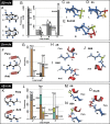
. 2015 Oct 6;112(40):E5478-85.
doi: 10.1073/pnas.1509508112. Epub 2015 Sep 22.

Control over overall shape and size in de novo designed proteins

Affiliations

Control over overall shape and size in de novo designed proteins

Yu-Ru Lin et al. Proc Natl Acad Sci U S A. .

Abstract

We recently described general principles for designing ideal protein structures stabilized by completely consistent local and nonlocal interactions. The principles relate secondary structure patterns to tertiary packing motifs and enable design of different protein topologies. To achieve fine control over protein shape and size within a particular topology, we have extended the design rules by systematically analyzing the codependencies between the lengths and packing geometry of successive secondary structure elements and the backbone torsion angles of the loop linking them. We demonstrate the control afforded by the resulting extended rule set by designing a series of proteins with the same fold but considerable variation in secondary structure length, loop geometry, β-strand registry, and overall shape. Solution NMR structures of four designed proteins for two different folds show that protein shape and size can be precisely controlled within a given protein fold. These extended design principles provide the foundation for custom design of protein structures performing desired functions.

Keywords: control protein shape; de novo design; ideal protein; protein design.


Conflict of interest statement

The authors declare no conflict of interest.

Figures
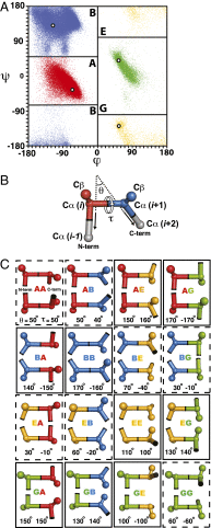
Fig. 1.
Fig. 1.
Discrete state model of protein local geometry. (A) ABEGO representation of protein local structure shown on Ramachandran plot. A, alpha region; B, beta region; G and E, positive phi region. The most frequently observed torsion angles for each region are indicated by the white circle. (B) Two-residue “lego blocks” are represented by four consecutive Cα atoms connected by virtual bonds. It is useful to consider the net change in chain direction θ and the net twist τ produced by each lego block. θ is the angle between the vector from Cα(i) to Cα(i-1) and the vector from Cα(i+1) to Cα(i+2), and τ, the dihedral angle defined by Cα(i-1), Cα(i), Cα(i+1), and Cα(i+2). (C) Two views of each of the 16 lego blocks built from the A, B, G, and E geometries indicated by the white circles in A. θ (Left) and τ (Right) are indicated at the bottom of the images. For simplicity, the gray parts in B are omitted. While the E residues and most of the G residues are generally Gly, to make the structural feature of the blocks clear, Cβ atoms are shown.
Fig. 2.
Fig. 2.
Common loop geometries for ββ-, βα-, and αβ-units in naturally occurring proteins. (A, F, and K) Secondary structure packing orientation definitions of ββ-, βα-, and αβ-units are illustrated. (B, G, and L) Loop-type distributions in naturally occurring protein structures for ββ-, βα-, and αβ-units for different loop lengths. The white portions of the histograms indicate other loop types. (CE, HJ, and MO) Examples of the most frequently observed loop types. (B) The GG and EA loops are frequent two-residue L-chirality loops and BAAGB is the only common R-chirality loop. (G) The AB loop is highly preferred for Para orientation. A “B” extension of an AB loop generates the most frequent Anti orientation loop type, BAB; the color coding in the histograms indicates such loop inheritance. GBB also has Anti orientation. (L) The two-residue loop used in designs is GB (SI Appendix, Fig. S2). Extension of the GB loop generates the AGB, GBB, and AGBB loops. GBA is also a common three-residue loop and it gives rise to the four-residue AGBA loop. The less frequent three-residue loop, BAA, extends to the four-residue BAAB loop.
Fig. 3.
Fig. 3.
Loop geometry controls secondary structure lengths and helix-sheet tilt angles in alpha-beta super secondary structure elements. (A and D) Schematics of the βαββ-units and the βαβ-units found in the ferredoxin-like fold and the Rossmann fold, respectively. (B) Helix length depends on the strand length. Multiple sequence-independent simulations of βαββ-unit folding were carried out with fixed loop types and different strand and helix lengths, and the frequencies of successful βαββ-unit folding were assessed. For different strand lengths, optimal folding of the structure occurs for different helix lengths. (C) Examples of four βαββ-units with the same loop types but different strand lengths and the corresponding optimal helix lengths. (E) Helix length depends on βα-loop type. Multiple sequence-independent simulations of βαβ-unit folding were carried out with a fixed αβ-loop type and strand lengths but different βα-loop types, and the frequencies of successful βαβ-unit folding with different helix lengths were determined. Different βα-loop types yield different optimal helix lengths. (F and G) BAB and GBB loops result in different optimal helix lengths. (H) The tilt angle Ω of the α-helix relative to the β-sheet for αβ-units. (I) The Ω angle depends on αβ-loop type. The angle distribution was calculated from βαββ-unit folding simulations with the BAB loop for the βα-unit, with strand lengths 7 and helix length 14.
Fig. 4.
Fig. 4.
Backbone blueprints and design models for ferredoxin-like folds and Rossmann2×2 folds with different sizes and shapes. The ferredoxin-like fold (AE) and the Rossmann2×2 fold (F and G). Backbone blueprint for each topology (Left) and a corresponding Rosetta generated backbone structure (Right). (A) Fd_5S: 58 residues, with register shift between the first and third strands. (B) Fd_5A: 66 residues, without register shift. (C) Fd_7S: 74 residues, with register shift. (D) Fd_7A: 76 residues, without register shift. (E) Fd_9A: 98 residues, without register shift. (F) Rsmn2×2_5: 87 residues. (G) Rsmn2×2_6: 99 residues. Helices are represented by pink or red rectangles, and strands by arrows with individual positions indicated by filled and open boxes. The filled boxes represent pleats coming out of the page, and the open boxes, pleats going into the page. Designed loop types are indicated for Fd_5S, Fd_5A, Fd_7S, Fd_9A, and Rsmn2×2_5. Fd_7A and Rsmn2×2_6 were designed by Koga et al. in 2012 (9), where they were referred as Di-I_5 and Di-II_10, respectively, using loop length but not loop type-based rules.
Fig. 5.
Fig. 5.
In silico energy landscapes and experimental characterization of designed proteins. (A) Energy landscapes obtained from Rosetta ab initio structure prediction simulations on Rosetta@home. Red points represent the lowest-energy structures obtained in independent Monte Carlo structure prediction trajectories starting from an extended chain for each sequence; y axis, Rosetta all-atom energy; x axis, Cα root mean square deviation (RMSD) from the design model. Green points represent the lowest-energy structures obtained in trajectories starting from the design model. (B) The far-UV circular dichroism (CD) spectra at various temperatures. (C) Chemical denaturation with GuHCl or urea monitored by CD at 220 nm at 25 °C. Urea was used for Fd_5A and Fd_7S denaturation and GuHCl for others. The data were fitted to a two-state model (red solid line) to obtain the free energy of unfolding ΔG. (D) Two-dimensional 1H-15N HSQC spectra at 25 °C and 600 MHz. p.p.m., parts per million.
Fig. 6.
Fig. 6.
Comparison of computational design models with experimentally determined NMR structures. (AF) Comparison of protein backbones of design models (Left) and NMR structures (Right); the Cα root mean square deviation (RMSD) between the two is indicated. (GJ) Comparison of core side-chain packing in superpositions of design models (rainbow) and NMR structures (gray). (A and G) Fd_5A_3 (2N2U). (B and H) Fd_7S_6 (2N2T). (D and I) Fd_9A_11 (2N76). (E and J) Rsmn2×2_5_6 (2N3Z). (C) Fd_7A_5 and (F) Rsmn2×2_6_10 designed by Koga et al. in 2012 (9) are included here for shape and size comparison.

References

    1. Tinberg CE, et al. Computational design of ligand-binding proteins with high affinity and selectivity. Nature. 2013;501(7466):212–216. - PMC - PubMed
    1. Chan WL, Zhou A, Read RJ. Towards engineering hormone-binding globulins as drug delivery agents. PLoS One. 2014;9(11):e113402. - PMC - PubMed
    1. Root MJ, Kay MS, Kim PS. Protein design of an HIV-1 entry inhibitor. Science. 2001;291(5505):884–888. - PubMed
    1. Fleishman SJ, et al. Computational design of proteins targeting the conserved stem region of influenza hemagglutinin. Science. 2011;332(6031):816–821. - PMC - PubMed
    1. Hume J, et al. Engineered coiled-coil protein microfibers. Biomacromolecules. 2014;15(10):3503–3510. - PubMed

Publication types