Rapid biotic homogenization of marine fish assemblages

Abstract

The role human activities play in reshaping biodiversity is increasingly apparent in terrestrial ecosystems. However, the responses of entire marine assemblages are not well-understood, in part, because few monitoring programs incorporate both spatial and temporal replication. Here, we analyse an exceptionally comprehensive 29-year time series of North Atlantic groundfish assemblages monitored over 5° latitude to the west of Scotland. These fish assemblages show no systematic change in species richness through time, but steady change in species composition, leading to an increase in spatial homogenization: the species identity of colder northern localities increasingly resembles that of warmer southern localities. This biotic homogenization mirrors the spatial pattern of unevenly rising ocean temperatures over the same time period suggesting that climate change is primarily responsible for the spatial homogenization we observe. In this and other ecosystems, apparent constancy in species richness may mask major changes in species composition driven by anthropogenic change.

Figure 1. Temporal trends in α diversity (rarefied species richness) and β diversity (Jaccard similarity, relative to the initial year), in each latitudinal band, over the duration of study.

Trend lines (OLS regression) are colour coded red if significantly negative (P<0.05, n=28) and grey if not significant. (There were no significant positive slopes). See Supplementary Figure 2 for overall trend.

Figure 2. Box plots (median, quartiles, range and outliers) of pairwise similarities (Jaccard) between latitudinal bands in each year of the study.

The trend line (OLS regression) is shown (r²=0.42, P<0.001). Years in which the mean pairwise similarity is below the overall mean are shown in red, and those above the mean in blue. (A similar pattern emerges if Bray–Curtis similarity is used. See Supplementary Figure 3).

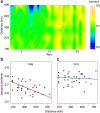
Figure 3. Similarity over space and time.

(a) Contour plot illustrating the relationship between Jaccard similarity and geographical distance (between latitudinal bands) over the duration of the study. The scale bar is to the right of the plot. The plot highlights increasing similarity through time, and greater homogenization across distant localities. (bottom) Distance-decay plots for an early ((b) 1986) and late ((c) 2013) year in the study. Median slopes shown. Distances (km) are between latitudinal bands. Compositional similarity of more distant localities increases through time (See Supplementary Figure 4 for further analysis of distance decay).

Figure 4. Similarity and temperature.

(a) Mean oceanographic surface temperature (depth<10 m) data in the first quarter of the year for the study area, in relation to year. The plot shows an increase in mean temperature through time (OLS regression, r²=0.22, n=162). (b) Relationship between temperature and latitude ignoring year, indicating that, on average, water temperature is cooler in more northern localities. (c) Box plot (median, quartiles, range and outliers) of pairwise temperature differences between latitudinal bands (analogous to the plot in Figure 2). Years in which the mean pairwise difference is below the overall mean are shown in red, and those above the mean in blue. There is a significant negative correlation (Spearman r_s=−0.46, P=0.026, n=23) between mean annual temperature difference (this plot) and mean annual Jaccard dissimilarity (1-Jaccard). This indicates that the reduction in temperature difference parallels the reduction in differences in community composition. (d) Median slope of the relationship between temperature and latitude in each year of the study showing the steepness of the temperature gradient is declining over time. This trend is significant (Spearman r_s=0.6, P=0.001, n=27).

References

1. Jackson J. B. C. The future of the oceans past. Philos TransR Soc B: Biol. Sci. 365, 3765–3778 (2010). - PMC - PubMed
1. Corlett R. T. The Anthropocene concept in ecology and conservation. Trends Ecol Evol 30, 36–41 (2015). - PubMed
1. Newbold T. et al. Global effects of land use on local terrestrial biodiversity. Nature 520, 45–50 (2015). - PubMed
1. McGill B. J., Dornelas M., Gotelli N. J. & Magurran A. E. Fifteen forms of biodiversity trend in the Anthropocene. Trends Ecol Evol 30, 104–113 (2015). - PubMed
1. Vellend M. et al. Global meta-analysis reveals no net change in local-scale plant biodiversity over time. Proc. Natl Acad. Sci. USA 110, 19456–19459 (2013). - PMC - PubMed
Publication types