Simple Learned Weighted Sums of Inferior Temporal Neuronal Firing Rates Accurately Predict Human Core Object Recognition Performance

Abstract

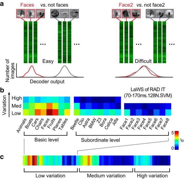
To go beyond qualitative models of the biological substrate of object recognition, we ask: can a single ventral stream neuronal linking hypothesis quantitatively account for core object recognition performance over a broad range of tasks? We measured human performance in 64 object recognition tests using thousands of challenging images that explore shape similarity and identity preserving object variation. We then used multielectrode arrays to measure neuronal population responses to those same images in visual areas V4 and inferior temporal (IT) cortex of monkeys and simulated V1 population responses. We tested leading candidate linking hypotheses and control hypotheses, each postulating how ventral stream neuronal responses underlie object recognition behavior. Specifically, for each hypothesis, we computed the predicted performance on the 64 tests and compared it with the measured pattern of human performance. All tested hypotheses based on low- and mid-level visually evoked activity (pixels, V1, and V4) were very poor predictors of the human behavioral pattern. However, simple learned weighted sums of distributed average IT firing rates exactly predicted the behavioral pattern. More elaborate linking hypotheses relying on IT trial-by-trial correlational structure, finer IT temporal codes, or ones that strictly respect the known spatial substructures of IT ("face patches") did not improve predictive power. Although these results do not reject those more elaborate hypotheses, they suggest a simple, sufficient quantitative model: each object recognition task is learned from the spatially distributed mean firing rates (100 ms) of ∼60,000 IT neurons and is executed as a simple weighted sum of those firing rates. Significance statement: We sought to go beyond qualitative models of visual object recognition and determine whether a single neuronal linking hypothesis can quantitatively account for core object recognition behavior. To achieve this, we designed a database of images for evaluating object recognition performance. We used multielectrode arrays to characterize hundreds of neurons in the visual ventral stream of nonhuman primates and measured the object recognition performance of >100 human observers. Remarkably, we found that simple learned weighted sums of firing rates of neurons in monkey inferior temporal (IT) cortex accurately predicted human performance. Although previous work led us to expect that IT would outperform V4, we were surprised by the quantitative precision with which simple IT-based linking hypotheses accounted for human behavior.

Keywords: IT cortex; V4; categorization; identification; invariance; object recognition.

Figure 1.

a, Object recognition tasks. To explore a natural distribution of shape similarity, we started with eight basic-level object categories and picked eight exemplars per category resulting in a database of 64 3D object models. To explore identity preserving image variation, we used ray-tracing algorithms to render 2D images of the 3D models while varying position, size, and pose concomitantly. In each image, six parameters (horizontal and vertical position, size, rotation around the three cardinal axes) were randomly picked from predetermined ranges (see Materials and Methods). The object was then added to a randomly chosen background. All test images were achromatic. Human observers performed all tasks using an 8-way approach (i.e., see one image, choose among eight; see Materials and Methods). Two kinds of object recognition tasks were tested: basic-level categorization (e.g., “car” vs “not car”) and subordinate identification (e.g., “car 1” vs “not car 1”). We characterized performance for each of eight binary tasks (e.g., “animals” vs “not animals,” “boats” vs “not boats,” etc.) in each 8-way recognition block at two to three levels of variation, resulting in 64 behavioral tests (64 d′ values). b, Possible outcomes for each tested linking hypothesis. We defined multiple candidate neuronal and computational linking hypotheses (Fig. 5), determined the predicted (i.e., cross-validated) object recognition accuracy (d′) of each linking hypothesis on the same 64 tests (y-axis in each scatter plot), and compared those results with the measured human d′ (x-axis in each scatter plot). A priori, each tested linking hypothesis could produce at least four possible types of outcomes. The pattern of predicted d′ might be unrelated to or strongly related to human d′ (left vs right scatter plots). We quantified that by computing consistency, the correlation between predicted d′ and actual human d′ across all 64 object recognition tests. Average predicted d′ might be low or matched to human d′ (bottom vs top scatter plots). We quantified performance by computing the median ratio of predicted d′ and actual human d′, across all 64 object recognition tests. For brevity, we will refer to these two metrics as consistency and performance from here on. Our goal was to find at least one “sufficient” code: a linking hypothesis that perfectly predicted the human d′ results on all object recognition tests (top right scatter plot).

Figure 2.

Neural responses. a, We used multielectrode arrays to record neural activity from two stages of the ventral visual stream [V4 and IT (PIT + CIT + AIT)] of alert rhesus macaque monkeys. We recorded neural responses to the same images used in our human psychophysical testing. Each image was presented multiple times (typically ∼50 repeats, minimum 28) using standard rapid visual stimulus presentation (RSVP). Each stimulus was presented for 100 ms (black horizontal bar) with 100 ms of neutral gray background interleaved between images. Although some of our neural sites represented single neurons, the majority of our responses were multiunit (see Fig. 8a). The rasters for repeated image presentations were then tallied within a defined time window (e.g., 70–170 ms after image onset, red rectangle, black vertical line indicated stimulus onset) to compute an average firing rate in impulses per second. The mean evoked firing rate is an entry in a response vector (green vertical vector, green saturation is proportional to response magnitude) that summarizes the population response to a single image. The concatenation of the response vectors produces a response matrix representing the population neural response of a particular visual area to our database of 5760 images. We parsed our neural population into V4 and IT, treating the various parts of IT as one population. We recorded from 168 neural sites in IT and 128 neural sites in V4. b, Approximate placement of the arrays in V4 (green shaded areas) and IT (blue shaded area) is illustrated by the black squares on two line drawings representing the brains of our two subjects.

Figure 3.

Human core object recognition results. a, Each color matrix from left to right summarizes the pooled human d′ for each of the three task sets ranging from basic level categorization to subordinate level face identification. In each matrix, the amount of identity preserving image variation was increased from low (bottom) to high (top), resulting in a total of 64 behavioral tests. Red represents high performance (d′ = 5) and blue low performance (d′ = 0). For each 8-way test set and each level of variation, the computed eight d′s were based on the average confusion matrix of multiple observers (basic level categorization, n = 29, car identification, n = 39, face identification, n = 40; see Materials and Methods for more information). b, Human to human consistency. The scattergram shows the performance (d′) of one human observer plotted against the performance (d′) of the pooled population of human observers across all 64 tests. The individual human observer was created by randomly combining the performance of three subjects on the three test sets (basic-level categorization and car and face subordinate-level identification). The population performance was computed based on a confusion matrix that combined the judgment of our entire pool (n = 104) of human observers. The Spearman correlation coefficient in this example was 0.941 (with a 68% CI = [0.921, 0.946] over the choice of behavioral tests). Median relative performance was 0.999 (with a test-induced 68% CI = [0.965, 1.073] over the choice of behavioral tests). c, Example images. Each octet of images are image samples representing all eight objects used for each of the three tested task sets at three example variation levels: basic level categorization (high variation), car identification (low variation), face identification (medium variation).

Figure 4.

Predicted performance pattern of an example LaWS of RAD IT neuronal linking hypothesis. In this example, the hypothesized neural activity that underlies behavior is as follows: in IT, from 128 units, mean firing rate, in a time window of 70–170 ms; and the decoder is an SVM decoder. a, Based on the aforementioned features of neural activity, a depiction of the outputs of two example decoders for two tasks from two different task sets. For each task set (basic categorization, subordinate identification) and each variation level (low, medium, high), we randomly divided our image responses into “training” and “testing” samples. We used the “training” samples, depicted by the green response vectors, to optimize eight “one-vs-rest” linear decoders. The performance of each decoder was then evaluated on the “testing” images. The red and black distributions summarize the response output of two such decoders to a sample of “testing” images. b, Predicted pattern of behavioral performance for all 64 behavioral tests. To generate these predictions, we constructed an 8-way decoder for each of the three task sets. Analogous to what the human observers were asked to do, for each task set, we applied all eight decoders and scored the decoder with the largest output margin as the behavioral “choice” of the linking hypothesis. Our final d′s are the average of at least 50 iterations of randomly picked train/test splits. Similar to Figure 3, the color matrices depict predicted performance (d′) for this example linking hypotheses for all task sets and variation levels (64 predicted d′ values). c, To facilitate comparison among different linking hypotheses and with human behavior (see Fig. 5), we strung out the color matrices into a color vector grouping task sets at each variation level.

Figure 5.

Candidate linking hypotheses. a, Candidate linking hypotheses that we explored were drawn from a space defined by four key parameters: spatial location of sampled neural activity, the temporal window over which the response of our units was computed (mean rate in this window), the number of units, and the type of hypothesized downstream decoder. Each candidate linking hypothesis is a specific combination of these parameters. For example, in green is a V4-based linking hypothesis with a temporal window of 70–170 ms that includes 128 neural sites and uses an SVM decoder. The predicted performance of each linking hypothesis for each behavioral test is depicted as a color vector where blue signifies low predicted performance (d′ = 0) and red signifies high predicted performance (d′ = 5). The goodness of each linking hypothesis can be visually evaluated by comparing its color pattern with that of the human population. b, Consistency. To quantify the ability of each linking hypothesis to predict the pattern of human performance (i.e., the similarity between color vectors in a), we computed the Spearman rank correlation coefficient between predicted performance and actual (pooled human, 104 subjects) across all task d′s. Median human-to-human correlation is indicated by the dashed line (median Spearman correlation coefficient of 0.929). The gray region signifies the range of human-to-human consistency (68% CI = [0.882, 0.957]). Each bar represents a different candidate linking hypothesis (bar length is proportional to task-induced variability). For pixel features (open symbol), V1-like features (filled black symbol), and computer vision features (red filled symbols), we picked the linking hypothesis that performed best. For neural features (V4 (green) and IT (blue), we matched the number of units at 128. Only bars that enter the gray region correspond to linking hypotheses that successfully predict human behavior. Within the context of IT-based linking hypothesis, we explored finer grain temporal codes (c). We also took advantage of our simultaneous multielectrode array recording to assess the impact of trial-by-trial firing rate correlation on the pattern of performance predicted by our most successful linking hypothesis (d). We considered the idea of a modular IT linking hypothesis with different subregions of IT being devoted exclusively to certain kinds of tasks (e). First, we compared the performance of “face patch” sites to “nonface patch” sites on all tests. We then stitched together an “expert linking hypothesis” in which each test is performed by neuronal sites that are tailored to that test (e.g., “face” detection is only done by “face neurons” whereas “car” detection is done by nonface neurons). To be complete, we compared the performance of our different modular IT linking hypotheses on both face tests only (n = 17 of the 64 tests) and nonface tests only. As in b, pattern of performance was always compared with human-to-human consistency indicated by the gray region.

Figure 6.

Exploring a large set of linking hypotheses. The y-axis shows consistency (defined in Fig. 5b) and the x-axis shows performance—the median of the ratio between predicted and actual (human) d′ across all 64 tests. In total, we tested 944 types of linking hypotheses, varying the number of neurons/features in each case, for a grand total of 50,685 instantiations considered. Here, we show the results of 755 of those hypotheses. The result of each specific instantiation is shown as a point in the plot with color used to indicate the “spatial” location of the features (IT, V4, V1, or computer vision). We show these examples to illustrate the parameters that we varied, which included spatial location, temporal window, number of units, type of decoder, and a variety of training procedures and train/test splits (see Fig. 10a). The horizontal dashed line indicates the average human-to-human consistency and the horizontal gray band represents variability in human-to-human consistency. The vertical dashed line indicates the average relative human-to-human performance and by definition is at 1 and the vertical gray band shows the human-to-human variability in relative performance. Any linking hypothesis that falls in the red dashed circle is perfectly predicting human performance on these 64 tests. Note that much of the scatter in the IT-based linking hypotheses (blue) is due to varying the number of neural sites, as illustrated in Figure 7b.

Figure 7.

Effect of number of units and temporal window on consistency and performance. Here, we show the results for the LaWS of RAD linking hypotheses (see text), but results are qualitatively similar for other hypotheses. a, Scattergrams show predicted performance (d′) for two neuronal linking hypotheses, IT (blue) and V4 (green), plotted against the actual human performance on all 64 tests: low variation (open circles), medium and high variation (filled circles). The number of units increases from 16 neural sites (left) to 128 neural sites (right). For each linking hypothesis, we also computed its performance: the median of the ratio between predicted and actual human performance across all d′s for all 64 tests. b, Performance (defined in Fig. 6) versus consistency for the V4- and IT-based linking hypotheses as a function of the number of (trial-averaged) units. The curve fits are [IT, r² = 0.996; V4, r² = 0.91] and they predict that ∼529 IT trial-averaged neural sites and ∼22,096 V4 trial-averaged neural sites would match human performance under the LaWS of RAD linking hypothesis. c, Consistency for different temporal windows of reading the neural activity. Each point is computed with a 100-ms-wide window and the x-axis shows the center of that window. The number of trial-averaged neural sites was fixed at 128. d, Consistency versus performance for the LaWS of RAD IT linking hypothesis at several progressive temporal windows with the center location starting at the time of image onset (0 ms) and up to 500 ms after image onset. The width of the temporal window was fixed at 100 ms (code details are same as b, except the number of trial-averaged neural sites was fixed at 128).

Figure 8.

a, SUA versus MUA linking hypotheses. We used a profile-based spike sorting procedure (Quiroga et al., 2004) and an affinity propagation clustering algorithm (Frey and Dueck, 2007) to isolate the responses of 16 single units from our sample of 168 IT neuronal sites. The minimum signal-to-noise ratio (SNR) for each single unit cluster was set to 3.5, with SNR defined as the amplitude of the mean spike profile divided by root mean square error (RMSE) across time points. Consistency with the human pattern of performance versus performance for SUA (red) and MUA (black). We estimate that twice as many neurons are needed so that the consistency-performance relationship of our SUA linking hypothesis matches that of our MUA linking hypothesis. All parameters and training procedures of SUA- and MUA-based linking hypotheses were identical (performance was based on the average of five repetitions using a CC in which the units were randomly divided into nonoverlapping groups to estimate error from independent sampling of units). b, Single trial versus averaged trials linking hypotheses. Because human subjects were asked to make judgements on single image presentations, we also explored a “single trial” training and testing analysis in which we treated the responses of the neural units to each images presentation as a new and independent set of neural units (i.e., “unrolled” the trial dimension into the unit dimension). Consistency versus performance for the single-trial (red) and the averaged-trial (black) LaWS of RAD linking hypotheses (based on a correlation decoder). We estimate that ∼60 times as many neurons are needed so that the consistency-performance relationship of our single-trial linking hypothesis matches that of our averaged-trials linking hypothesis. Error bars are SDs induced by independent sampling of units as in a.

Figure 9.

No significant difference in consistency and performance of IT subpopulations was seen when parsed based on anatomical subdivision: PIT versus CIT versus AIT. Based on anatomical landmarks, we could conservatively divide our population of 168 IT neural sites into the following: 76 in PIT, 75 in CIT, and 17 in AIT. a, Comparison of the consistency values for IT populations when neural sites respected anatomical boundaries (PIT vs CIT vs AIT) in contrast to a “control” populations in which the sites were randomly picked from all three anatomical subdivisions. There was no significant difference between the IT populations regardless of whether we restricted our population to 17 neural sites (limiting our analysis to the number of neural sites in AIT our least sampled anatomical subdivision) or expanded to 75 neural sites and compared PIT and CIT. Similarly, performance (b) showed no significant differences between the different IT populations. It is important to note that the decrease in consistency and neural performance is expected based on the smaller population sizes (see Fig. 7b). Consistency and performance were computed based on our typical 70–170 temporal window using an SVM decoder.

Figure 10.

a, Effect of the training procedure. Shown are consistency values for LaWS of RAD V4 and IT linking hypotheses under different training procedures. The number of units was fixed to 128 units and the temporal window was 70–170 ms after the onset of the image presentation. Two types of decoders were tested (SVMs and CCs). We also varied the number of images used to train the decoder (leave-2-out: for each class, all images but two were used as the training set and the remaining two were used for testing; 80%: 80% of images were used for training, and the held-out 20% were used for testing; 20%: similar to 80%, but 20% were used for training and 80% for testing). In the blocked training regime, the training and testing of a decoder was done for each variation level separately. For the unified training regime, the decoders were trained across all variations and tested on each variation level separately. b, Trade-off between the sufficient number of units and the number of training images per object for the LaWS of RAD IT linking hypothesis (in which the temporal window was fixed at 70–170 ms and SVM decoders were used). In each data point, the performance of the linking hypothesis was projected to reach the human-to-human consistency (within the subject-to-subject variability) and the human absolute performance (relative performance of one). On the y-axis, the numbers shown in black indicate the projected number of repetition-averaged, multiunit neural sites that are sufficient and the numbers in red indicate the number of single-trial, single-unit sites that are sufficient (120× larger). For example, the asterisk indicates a LaWS of RAD IT linking hypothesis of ∼60,000 single units discussed above and the plot shows that it would require ∼40 training examples per object to learn de novo (with a 68% CI of ∼[30, 60]; data not shown in the plot).

References

1. Afraz SR, Kiani R, Esteky H. Microstimulation of inferotemporal cortex influences face categorization. Nature. 2006;442:692–695. doi: 10.1038/nature04982. - DOI - PubMed
1. Afraz A, Boyden ES, DiCarlo JJ. Optogenetic and pharmacological suppression of spatial clusters of face neurons reveal their causal role in face gender discrimination. Proc Natl Acad Sci U S A. 2015;112:6730–6735. doi: 10.1073/pnas.1423328112. - DOI - PMC - PubMed
1. Averbeck BB, Latham PE, Pouget A. Neural correlations, population coding and computation. Nat Rev Neurosci. 2006;7:358–366. doi: 10.1038/nrn1888. - DOI - PubMed
1. Biederman I, Gerhardstein PC. Recognizing depth-rotated objects: evidence and conditions for three-dimensional viewpoint invariance. J Exp Psychol Hum Percept Perform. 1993;19:1162–1182. doi: 10.1037/0096-1523.19.6.1162. - DOI - PubMed
1. Biederman I, Gerhardstein PC, Cooper EE, Nelson CA. High level object recognition without an anterior inferior temporal lobe. Neuropsychologia. 1997;35:271–287. doi: 10.1016/S0028-3932(96)00075-9. - DOI - PubMed
Publication types
LinkOut - more resources