Acoustic holography as a metrological tool for characterizing medical ultrasound sources and fields

Abstract

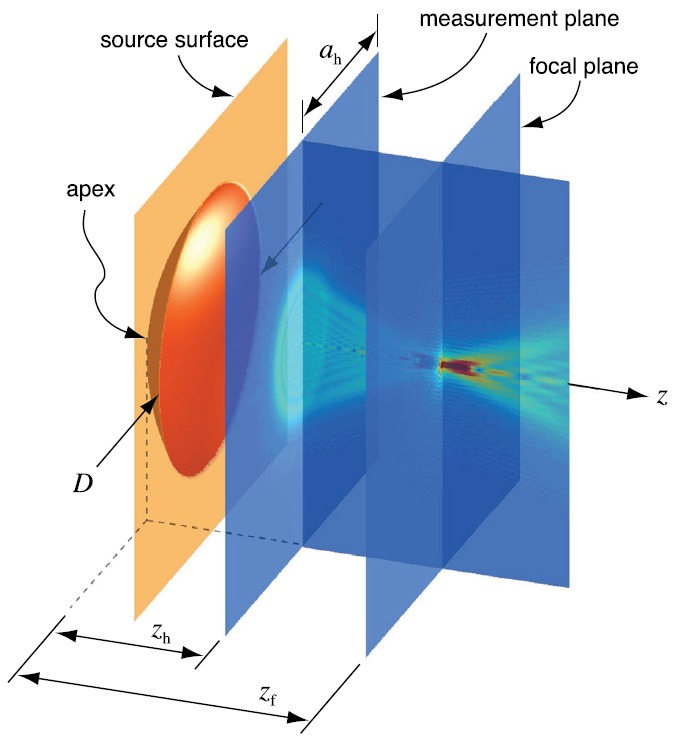
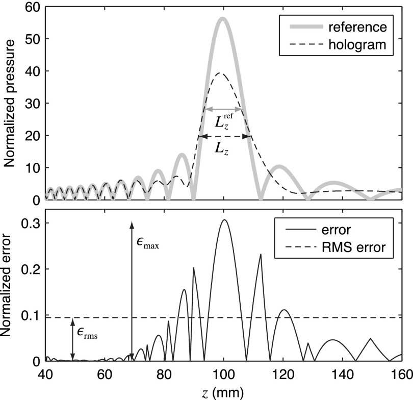
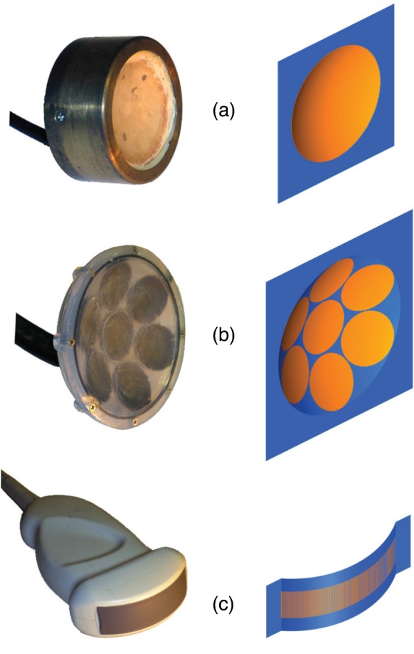
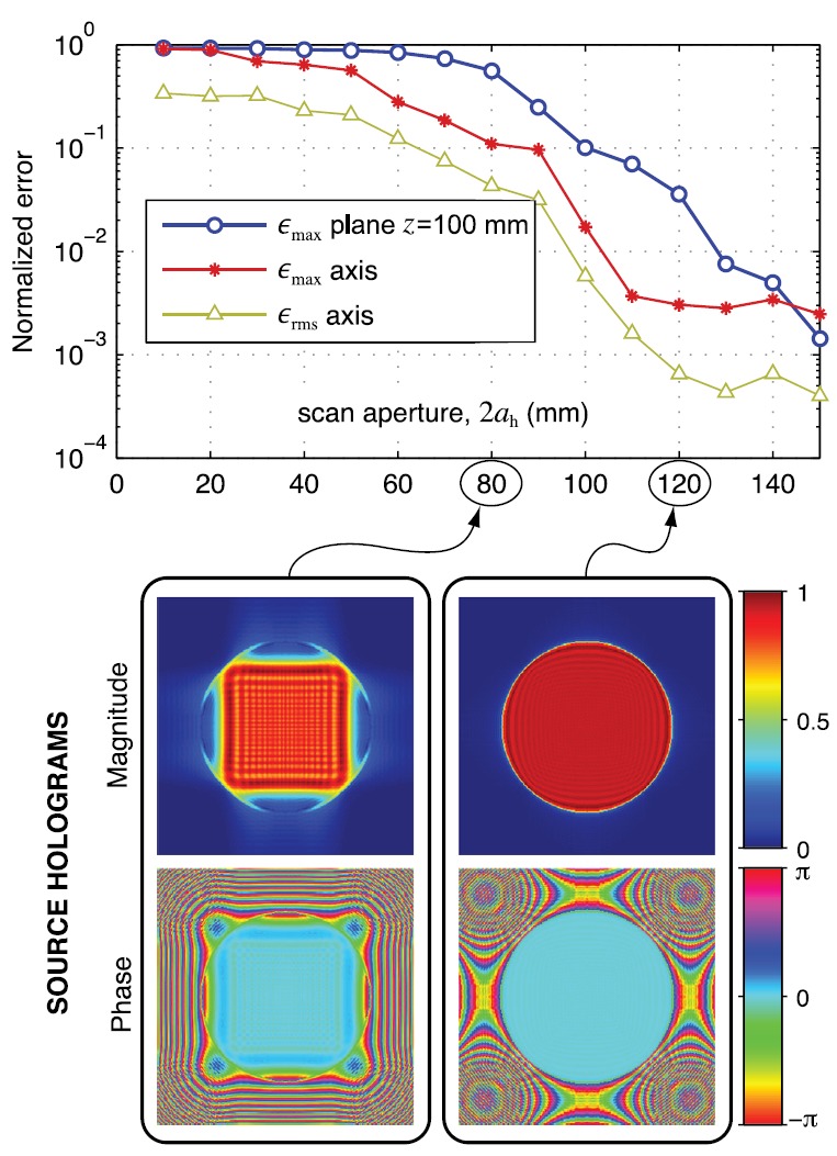
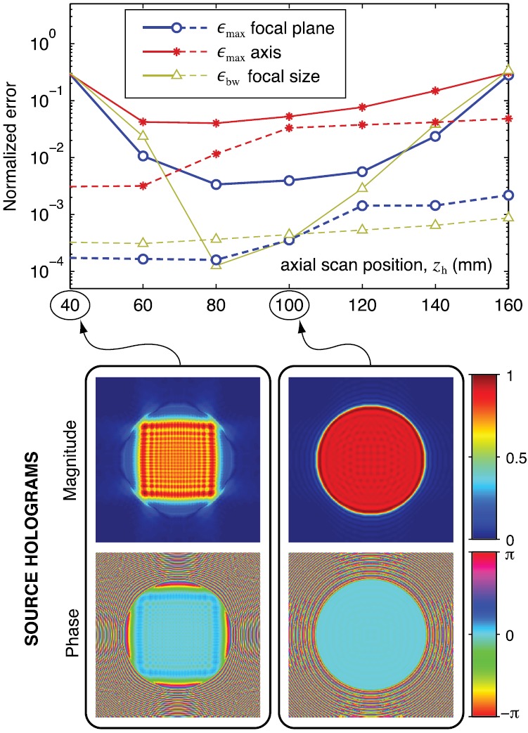
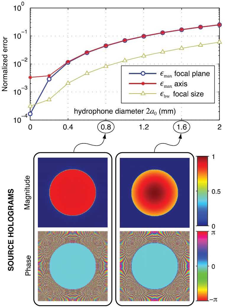
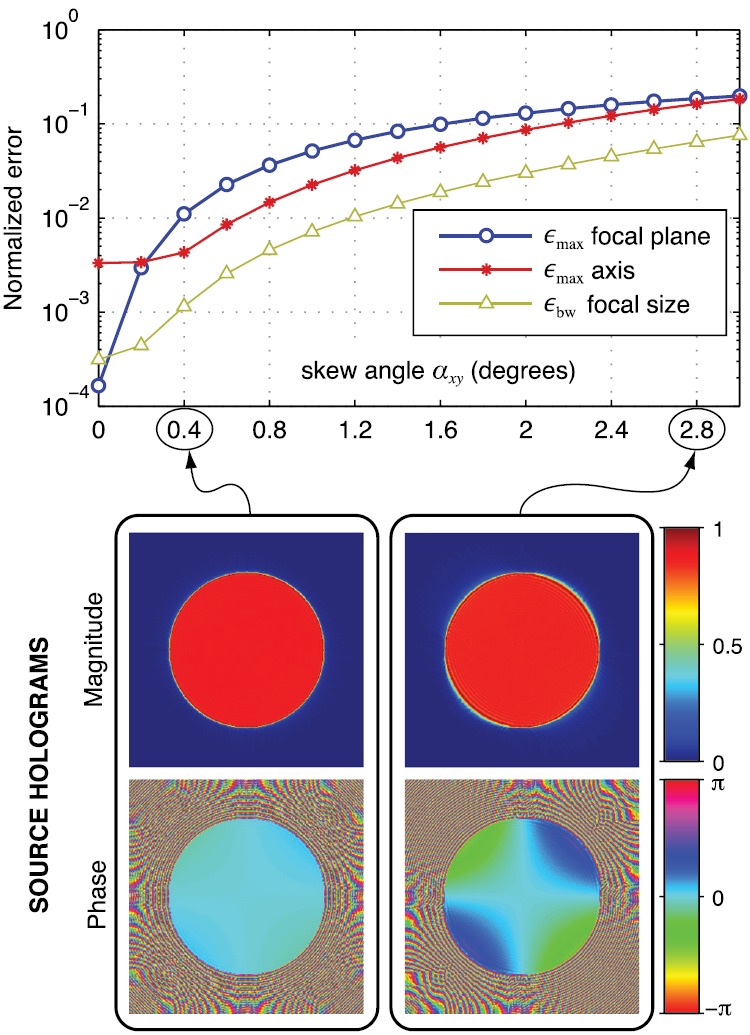
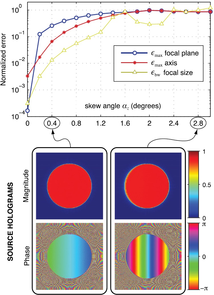
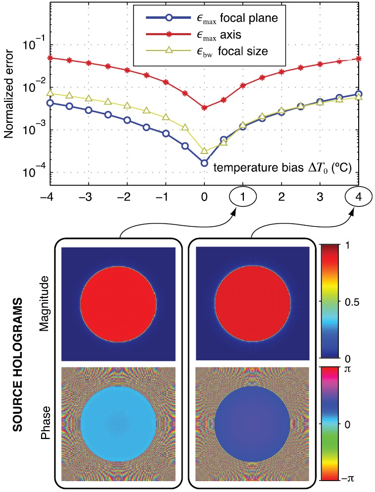
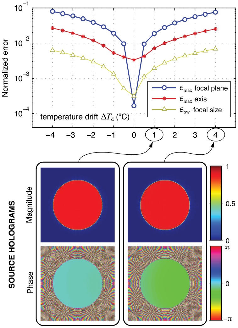
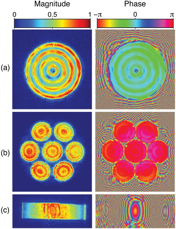
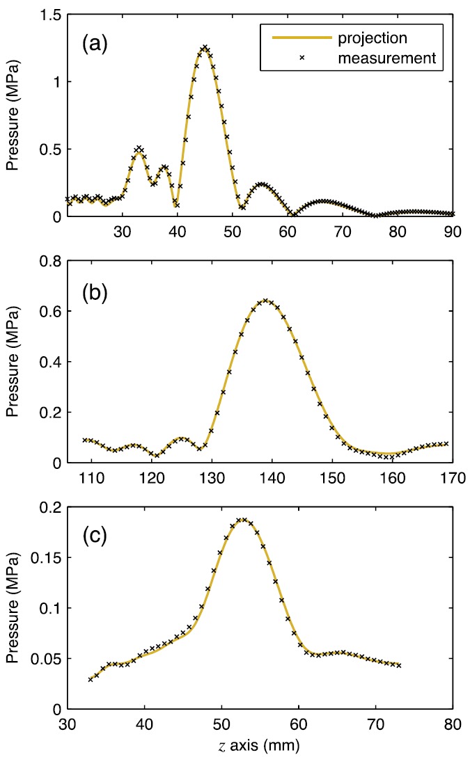
Acoustic holography is a powerful technique for characterizing ultrasound sources and the fields they radiate, with the ability to quantify source vibrations and reduce the number of required measurements. These capabilities are increasingly appealing for meeting measurement standards in medical ultrasound; however, associated uncertainties have not been investigated systematically. Here errors associated with holographic representations of a linear, continuous-wave ultrasound field are studied. To facilitate the analysis, error metrics are defined explicitly, and a detailed description of a holography formulation based on the Rayleigh integral is provided. Errors are evaluated both for simulations of a typical therapeutic ultrasound source and for physical experiments with three different ultrasound sources. Simulated experiments explore sampling errors introduced by the use of a finite number of measurements, geometric uncertainties in the actual positions of acquired measurements, and uncertainties in the properties of the propagation medium. Results demonstrate the theoretical feasibility of keeping errors less than about 1%. Typical errors in physical experiments were somewhat larger, on the order of a few percent; comparison with simulations provides specific guidelines for improving the experimental implementation to reduce these errors. Overall, results suggest that holography can be implemented successfully as a metrological tool with small, quantifiable errors.

FIG. 1.

(Color online) Schematic of the relevant geometry. A source with its apex located at the z-axis origin radiates a beam in the $+z$ direction. From this beam, a planar hologram with aperture $2a_{\mathrm{h}}$ is measured at $z=z_{\mathrm{h}}$. This measured hologram is then backprojected to a source surface that comprises the surface of the physical transducer in conjunction with a plane that extends outward from the transducer aperture D. Forward projection from the source hologram can then reconstruct the full 3D field.

FIG. 2.

Definition of holographic reconstruction errors for a collection of points. The top plot shows the axial distribution of pressure magnitude for a uniform, focused source as determined by reference calculations and field reconstruction from a hologram. The −6 dB “beamwidth” corresponding to each field is labeled; these values are used to calculate the error metric ${\mathrm{ϵ}}_{\text{bw}}$. The bottom plot shows the deviation between the two fields in terms of both a peak value ${\mathrm{ϵ}}_{\text{max}}$ and an average value ${\mathrm{ϵ}}_{\text{rms}}$. Both of these error metrics are normalized by the maximum reference pressure magnitude over the collection of points considered.

FIG. 3.

(Color online) Photographs of transducers used in experiments along with depictions of the surfaces on which source holograms were reconstructed. For visual clarity, transducer elements expected to vibrate are depicted on the surfaces of (a) a single-element focused source (2.2 MHz, aperture 45 mm, F-number 1); (b) a focused transducer comprising 7 elements (1 MHz, aperture 147 mm, F-number 0.95); and (c) a convex imaging probe with 128 elements (2.3 MHz, aperture 49.9 × 13.5 mm, elevational lens with approximate focal distance of 50 mm).

FIG. 4.

(Color online) Field reconstruction errors (top) for the flat source (100 mm aperture) as a function of the size of the measurement region. This region is a square $2a_{\mathrm{h}}\times 2a_{\mathrm{h}}$ with its center placed on the acoustic axis at $z_{\mathrm{h}}=50$ mm. Bottom images illustrate the reconstructed source hologram in terms of velocity magnitude and phase distributions for two possible sizes of the measurement region (corresponding measurement apertures are circled).

FIG. 5.

(Color online) Field reconstruction errors (top) for the focused source (100 mm aperture) as a function of the axial position $z_{\mathrm{h}}$ of the measurement region. Solid lines correspond to a measurement region with aperture $2a_{\mathrm{h}}=50$ mm; dashed lines correspond to a region with aperture $2a_{\mathrm{h}}=150$ mm. Bottom images illustrate source holograms reconstructed using the smaller measurement aperture at the indicated axial measurement positions.

FIG. 6.

(Color online) Field reconstruction errors (top) for the focused source as a function of the diameter of the hydrophone's sensing element. The measurement region is located at $z_{\mathrm{h}}=50$ mm with aperture $2a_{\mathrm{h}}=150$ mm. Bottom images illustrate reconstructed source holograms for the indicated hydrophone diameters.

FIG. 7.

(Color online) Field reconstruction errors (top) for the focused source as a function of the skew angle relative to 90° of the transverse $x\prime y\prime$ coordinate axes used in capturing measurements within the scan plane. The measurement region is at $z_{\mathrm{h}}=50$ mm with aperture $2a_{\mathrm{h}}=150$ mm. Bottom images illustrate reconstructed source holograms for the indicated skew angles.

FIG. 8.

(Color online) Field reconstruction errors (top) for the focused source as a function of the angular misalignment between the source's acoustic axis and the direction normal to the scan plane. The measurement region is at $z_{\mathrm{h}}=50$ mm with aperture $2a_{\mathrm{h}}=150$ mm. Bottom images illustrate reconstructed source holograms for the indicated misalignment angles.

FIG. 9.

(Color online) Field reconstruction errors (top) for the focused source as a function of the uncertainty in temperature at which the field measurements were made. This uncertainty is presumed to comprise a constant bias in the sound speed used in reconstructing the source hologram. The measurement region is located at $z_{\mathrm{h}}=50$ mm with aperture $2a_{\mathrm{h}}=150$ mm. Bottom images illustrate reconstructed source holograms for the indicated temperature biases.

FIG. 10.

(Color online) Field reconstruction errors (top) for the focused source as a function of the amount of temperature drift that occurs during the acquisition of measurements by a raster scan. Temperature is assumed to change linearly with the scan point number. The measurement region is at $z_{\mathrm{H}}=50$ mm with aperture $2a_{\mathrm{h}}=150$ mm. Bottom images illustrate reconstructed source holograms for the indicated temperature changes.

FIG. 11.

(Color online) Source holograms reconstructed from experimental measurements for the three sources depicted in Fig. 3. Note that velocity magnitudes are normalized relative to the maximum value in the hologram.

FIG. 12.

(Color online) Comparison of axial fields measured directly versus those projected from a measured hologram for the three sources depicted in Fig. 3.

FIG. 13.

(Color online) As used for field projection calculations, two surfaces ${\Sigma }_1$ and ${\Sigma }_2$ are depicted schematically relative to a coordinate system with origin O. Each surface corresponds to the locus of points represented by position vectors ${\mathbf{r}}_1$ or ${\mathbf{r}}_2$, respectively. ${\Sigma }_1$ represents a boundary surface with an acoustic source that radiates waves into the half-space region that includes ${\Sigma }_2$. This surface is further described by the outward facing unit normal ${\mathbf{n}}_1$ and differential area elements $d{\Sigma }_1$. ${\Sigma }_2$ is described by analogous notation and represents a non-physical surface at which field measurements are made.

References

1. Gabor D., “ Light and information,” in Progress in Optics, edited by Wolf E. ( North Holland, Amsterdam, 1961), Vol. 1, pp. 109–153.
1. Maynard J. D., Williams E. G., and Lee Y., “ Nearfield acoustic holography: I. Theory of generalized holography and the development of NAH,” J. Acoust. Soc. Am. 78(4), 1395–1413 (1985)10.1121/1.392911. - DOI
1. Williams E. G., Fourier Acoustics: Sound Radiation and Nearfield Acoustical Holography ( Academic, San Diego, CA, 1999), Chaps. 3, 5, 7.
1. Stepanishen P. R. and Benjamin K. C., “ Forward and backward projection of acoustic fields using FFT methods,” J. Acoust. Soc. Am. 71(4), 803–812 (1982).10.1121/1.387606 - DOI - PubMed
1. Schafer M. E. and Lewin P. A., “ Transducer characterization using the angular spectrum method,” J. Acoust. Soc. Am. 85(5), 2202–2214 (1989).10.1121/1.397869 - DOI
Publication types