Flexible gating of contextual influences in natural vision

Abstract

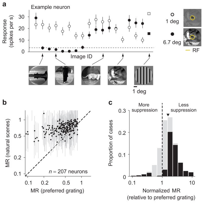
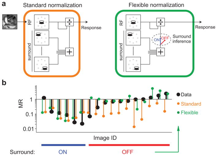
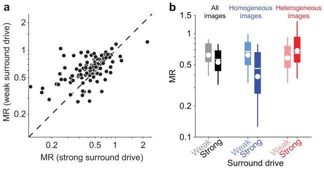
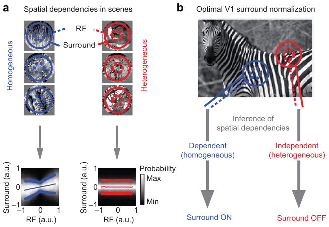
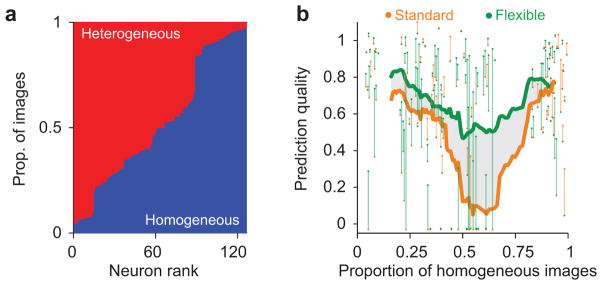
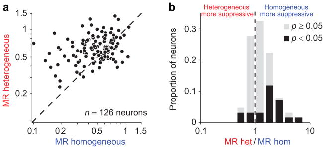
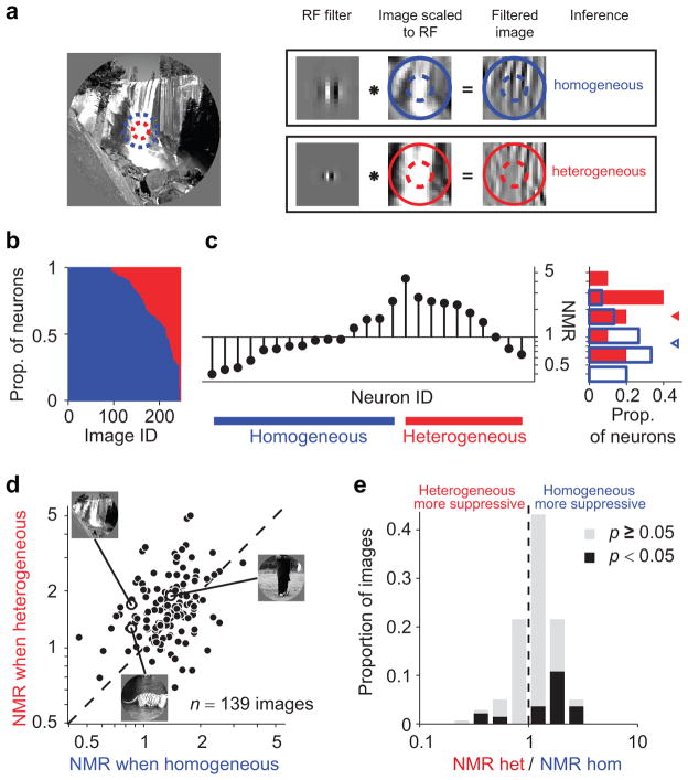
Identical sensory inputs can be perceived as markedly different when embedded in distinct contexts. Neural responses to simple stimuli are also modulated by context, but the contribution of this modulation to the processing of natural sensory input is unclear. We measured surround suppression, a quintessential contextual influence, in macaque primary visual cortex with natural images. We found that suppression strength varied substantially for different images. This variability was not well explained by existing descriptions of surround suppression, but it was predicted by Bayesian inference about statistical dependencies in images. In this framework, surround suppression was flexible: it was recruited when the image was inferred to contain redundancies and substantially reduced in strength otherwise. Thus, our results reveal a gating of a basic, widespread cortical computation by inference about the statistics of natural input.

Figure 1. Variability of surround modulation with natural images

(a) Firing rate of a V1 neuron in response to static natural images (circles), and gratings at the preferred orientation and spatial frequency (squares), windowed to 1 degree of visual space (open symbols) or 6.7 degrees (filled). The dashed line denotes the spontaneous rate. (b) Each point represents the modulation ratio (MR) measured with gratings at the preferred orientation and spatial frequency (abscissa) and the average MR across all natural images (ordinate), for each neuron. (c) Distribution of normalized MR (NMR) across all images and neurons (N = 38,591 cases). Arrowhead indicates geometric mean, black bars indicate cases with NMR significantly different from 1 (p < 0.05). Error bars in (a) indicate 68% c.i., in (b) standard deviations.

Figure 2. Standard and flexible normalization models of surround suppression

(a) Left: Schematic of the standard normalization model. Visual input is first passed through linear filters representing the RF (top left) and its surround (bottom left). Gray symbols denote the location of the center of each filter. The output of the RF filters is divided by the filters representing the RF and surround. Right: The flexible normalization model is identical to the standard normalization except that the surround can be turned on and off, on an image-by-image basis, depending on an inference about image homogeneity. (b) Black symbols, MR for each pair of responses shown in Fig. 1a; orange and green symbols, MR derived from the standard and flexible models, respectively, fit to the firing rates. In the flexible model, facilitation results when the surround stimulus provides additional drive to the RF, but surround suppression is inferred off.

Figure 3. Drive to the surround does not explain surround suppression strength

(a) Each point represents, for each neuron, the average MR for images which provide the surround with below average (ordinate) vs. above average (abscissa) drive. MR is only weakly modulated by surround drive, defined as the root mean square of the surround filters outputs. (b) Left pair: MR across all neurons, for images with weak vs. strong surround drive as in (a). Boxes denote the 25–75^th percentile; whiskers, 10–90^th percentile; white line, median; white circle, geometric mean. Middle and right pairs: same as the pair on the left, but including in the analysis only homogeneous (blue, light blue) or heterogeneous (red, pink) images.

Figure 4. Surround divisive normalization is optimal only for statistically homogeneous stimuli

(a) Left: Neighboring locations in homogeneous images contain redundant information. This produces a bowtie-shaped dependency in the outputs of filters representing the RF and surround. The dependency is illustrated in the conditional histogram (bottom): each column represents the histogram of surround filters’ outputs (position on the ordinate), given a particular output of the RF filters (abscissa). Lighter shades of gray indicate larger occurrence probability. Thin and thick lines represent conditional mean ± conditional standard deviation, respectively. Right: Neighboring locations in heterogeneous regions are independent, as evidenced by the absence of any structure in the conditional histogram (bottom). (b) Surround normalization reduces redundancy between RF and surround. Optimality requires that the normalization is turned off when the stimulus is heterogeneous. Schematic is adapted from ref. .

Figure 5. Standard and flexible normalization differ most for balanced image ensembles

(a) Proportion of images that were inferred homogeneous (blue) vs. heterogeneous (red, stacked bars), for each neuron. (b) Cross-validated prediction quality for the flexible (green) and standard (orange) models, as a function of the proportion of effective images that were inferred homogeneous. Each dot denotes the average prediction quality for an individual neuron. Each vertical line connects the prediction quality for the two models for each neuron, and is shaded green when the flexible model performed better and orange when it did not. Thick lines indicate a running average of the performance across neurons, including 30 data points, for each model. The shaded area denotes the difference in average prediction quality between flexible and standard models. The models performed similarly in cells driven primarily by homogeneous or heterogeneous images, but the flexible model performed much better in cells driven by balanced image ensembles.

Figure 6. Surround suppression strength depends on image homogeneity

(a) MR for heterogeneous vs. homogeneous images. Each symbol represents the average MR of a neuron, for each image class. (b) The ratio between MRs for the two image categories. Values larger than 1 correspond to neurons suppressed more by homogeneous than heterogeneous images. Black bars, neurons with a ratio significantly different from 1.

Figure 7. Homogeneity depends on neuronal tuning

(a) The same image (left) contains homogeneous structure for some neurons (RF position and size denoted with blue dashed circle; top), heterogeneous for others (red dashed circle; bottom). First column in the boxes: example filters representing two different neurons; second column: image patch scaled and centered to fit the RF; third column: the result of convolution between image and filter, indicating the image components visible to that filter. (b) Proportion of neurons for which a given image was inferred homogeneous (blue) vs. heterogeneous (red, stacked bars). Many images could be classified as either type, depending on the neuron’s tuning. (c) Stem plot: NMR for the example image in (a), across different neurons. Blue and red lines at the bottom denote neurons with surround inferred on and off, respectively. Bar plot: histogram of NMR values for each class. Triangles denote geometric mean. (d) Each symbol represents the NMR for an image, averaged separately when it was classified as heterogeneous (ordinate) or homogeneous (abscissa). Only images classified in both ways by at least 5% of neurons were included. (e) Distribution of the ratio between NMR in the two conditions. Images that were more suppressive when classified as homogeneous have values larger than 1. Black bars, images with ratios significantly different from 1.

References

1. Schwartz O, Hsu A, Dayan P. Space and time in visual context. Nat Rev Neurosci. 2007;8:522–535. - PubMed
1. Kohn A. Visual Adaptation: Physiology, Mechanisms, and Functional Benefits. J Neurophysiol. 2007;97:3155–3164. - PubMed
1. Carandini M, Heeger DJ. Normalization as a canonical neural computation. Nat Rev Neurosci. 2011;13:51–62. - PMC - PubMed
1. Li Z. Contextual influences in V1 as a basis for pop out and asymmetry in visual search. Proc Natl Acad Sci. 1999;96:10530–10535. - PMC - PubMed
1. Itti L, Koch C. Computational modelling of visual attention. Nat Rev Neurosci. 2001;2:194–203. - PubMed
Publication types
LinkOut - more resources