Biological Effects of Low-Frequency Shear Strain: Physical Descriptors

Abstract

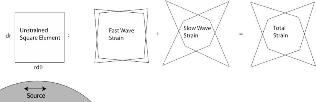
Biological effects of megahertz-frequency diagnostic ultrasound are thoroughly monitored by professional societies throughout the world. A corresponding, thorough, quantitative evaluation of the archival literature on the biological effects of low-frequency vibration is needed. Biological effects, of course, are related directly to what those exposures do physically to the tissue-specifically, to the shear strains that those sources produce in the tissues. Instead of the simple compressional strains produced by diagnostic ultrasound, realistic sources of low-frequency vibration produce both fast (∼1,500 m/s) and slow (1-10 m/s) waves, each of which may have longitudinal and transverse shear components. Part 1 of this series illustrates the resulting strains, starting with those produced by longitudinally and transversely oscillating planes, through monopole and dipole sources of fast waves and, finally, to the case of a sphere moving in translation-the simplest model of the fields produced by realistic sources.

Keywords: Acoustic dipole; Acoustic monopole; Biological effects; Low-frequency shear strain; Low-frequency vibration; Tactile perception; Transverse and longitudinal shear waves.

Figure 1

Realistic sources of low frequency vibration produce complex combinations of longitudinal and transverse, fast and slow waves in tissues. A sphere moving in translation produces all such fields. To help put these complex fields in perspective with simpler, more frequently studied examples, the discussion moves from plane waves through simple spherical fast waves (“Bubble”), fast dipole spherical waves (from two spherical sources with opposing phases), to the case of the translating sphere. Arrows show direction of motion of the source.

Figure 2

Displacements (left) and strains (right) given by eqn (3) and (5). μ = μ₁ + jωμ₂, where μ₁ = 1000 kPa and μ₂ =3 Pa s. Instantaneous values at t = 0 are solid, absolute values (amplitudes) are dashed. The normalized strain has units of reciprocal meters.

Figure 3

Tissue distortion expressed in eqn (5)–(7). The infinite plane source at x = 0, coming out of the page, oscillates up (upper) and down (lower) along the y-axis. An infinitesimal square (dotted) near the source in the cross-section is simultaneously rotated and strained into a diamond-shape. The rotation and strain have the same amplitudes and are directed so that their sum brings left face of the strained element back in line with the source giving us a parallelepiped for the total distortion of the element.

Figure 4

Normalized, absolute strain near a radially oscillating bubble S_rr (solid), S_θθ = S_ϕϕ (dashed), $\frac{\mathrm{\Delta }V}{V}$ (dotted). a=0.01 m, ω=1000 s⁻¹, ρ =1000 kg m⁻³, c_f =1500 m s⁻¹.

Figure 5

Normalized strain near the radially oscillating bubble of Figure 4. r = 0.02 m. All other parameters the same as Figure 4.

Figure 6

Normalized strain near a radially oscillating bubble. r = a + 0.01 m. All other parameters the same as Figure 4.

Figure 7

Normalized, absolute strain near an acoustic dipole. S_rr (solid), S_θθ = S_ϕϕ (dashed), $\frac{\mathrm{\Delta }V}{V}$ (dotted). ω=1000 s⁻¹, ρ =1000 kg m⁻³, c_f =1500 m s⁻¹, θ=0.

Figure 8

Normalized, absolute strain near a transversely oscillating sphere. S_rr (solid), S_θθ = S_ϕϕ (dashed), $\frac{\mathrm{\Delta }V}{V}$ (dotted), S_rθ (dot-dash), R (double dot-dash). a = 0.01 m, ω=1000 s⁻¹, c_f =1500 m s⁻¹, μ₁ = 3 kPa, μ₂ = 3 Pa s, ρ =1000 kg m⁻³, θ = π/4.

Figure 9

Normalized, absolute strain near a transversely oscillating sphere. S_rr (solid), S_θθ = S_ϕϕ (dashed), $\frac{\mathrm{\Delta }V}{V}$ (dotted), S_rθ (dot-dash). a = 0.01 m, r = 0.02 m, c_f =1500 m s⁻¹, μ₁ = 3 kPa, μ₂ = 3 Pa s, ρ =1000 kg m⁻³, θ = π/4.

Figure 10

Normalized, absolute strain near a transversely oscillating sphere. S_rr (solid), S_θθ = S_ϕϕ (dashed), $\frac{\mathrm{\Delta }V}{V}$ (dotted). r = a + 10 μ m, c_f =1500 m s⁻¹, μ₁ = 3 kPa, μ₂ = 3 Pa s, ρ=1000 kg m⁻³, θ = 0.

Figure 11

Original elements (white) of tissue at about 1 cm from the surface of a 1 cm sphere undergo shear strain (black), i.e., they change shape without change in volume, as the sphere moves forward. The longitudinal strain along the axis of oscillation is actually three-dimensional, i.e., as the axial dimension of the element changes both orthogonal dimensions change keeping the volume constant. At θ = π/2 shear is two dimensional, i.e., there are no azimuthal contributions to the shear strain along $\overrightarrow{e_{\varphi }}$ at θ = π/2. Parameters used in the computations are the same as those in Figures 7–9.

Figure 12

Strains attributable to fast and slow waves at 2 mm from the surface of a 1 cm sphere moving right and left with an amplitude of 1 mm. Solid and dotted parallelograms show the extremes of distortion of a square element of the medium. c_f =1500 m s⁻¹, c_s =1.7 m s⁻¹, i.e., μ₁ = 3 kPa, μ₂ = 0, ρ =1000 kg m³, ω = 1000 s⁻¹ (~160 Hz), θ = π/2, ξ₀ = 1 mm.

Figure 13

Using Oestreicher’s model of an oscillating sphere to illustrate the effects of contact area on strain. a = 1 mm: longitudinal (solid) and transverse (dotted). a = 2 cm: longitudinal (dashed) and transverse (dash-dotted). Abscissa d is distance from the surface of the vibrating sphere. μ₁ = 3000 kPa, μ₂ = 3 Pa s, ω = 2 π 160 s⁻¹.

Figure 14

Threshold for tactile perception at 250 Hz. Data from Verrillo (1980).

Figure 15

Threshold shifts resulting from exposure of the hand to accelerations of 20 m s⁻². Exposures were performed over a range of frequencies. The ordinate gives the ratio of post-exposure thresholds to their normal values. The dashed plot is the ratio for the 250 Hz threshold, the solid plot for the 16 Hz threshold. Frequency dependent thresholds were measured after each exposure. Figure adapted from Harada and Griffin (1991).

References

1. Békésy Gv. Über die Vibrationsempfindung. Akustische Zeitschrift. 1939;4:315–334.
1. Bell J, Bolanowski S, Holmes MH. The structure and function of Pacinian corpuscles: a review. Progress in neurobiology. 1994;42:79–128. - PubMed
1. Brisben AJ, Hsiao SS, Johnson KO. Detection of vibration transmitted through an object grasped in the hand. Journal of neurophysiology. 1999;81:1548–1558. - PubMed
1. Carstensen E, Gracewski SM, Dalecki D. Shear strain from irrotational tissue displacements near bubbles. J Acoust Soc Am. 2011;130:3467–3471. - PMC - PubMed
1. Carstensen E, Parker KJ. Oestreicher and elastography. J Acoust Soc Am. (in press). - PubMed
LinkOut - more resources