A process of rumour scotching on finite populations

Abstract

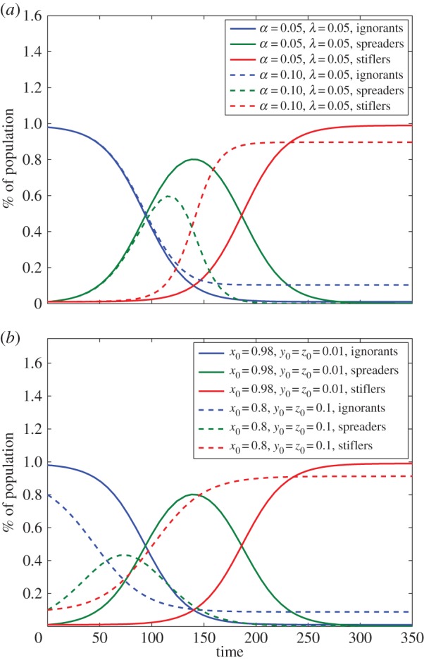
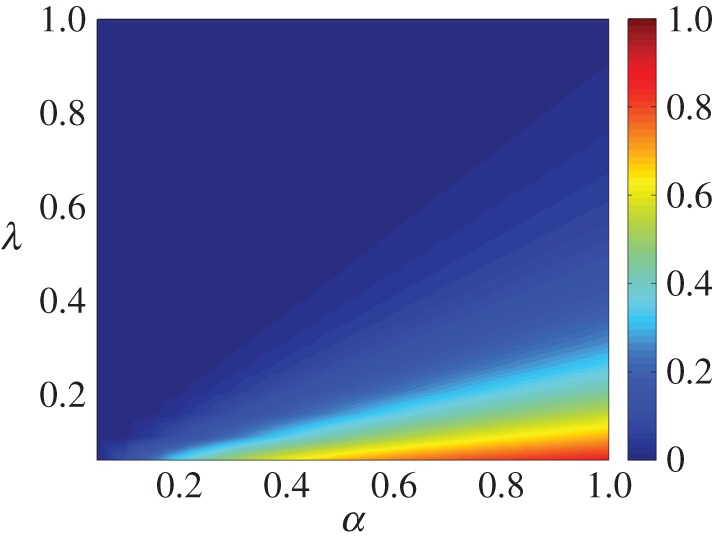
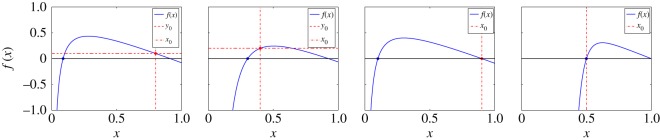
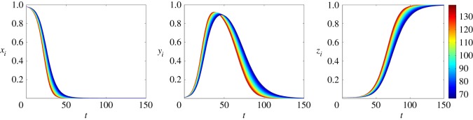
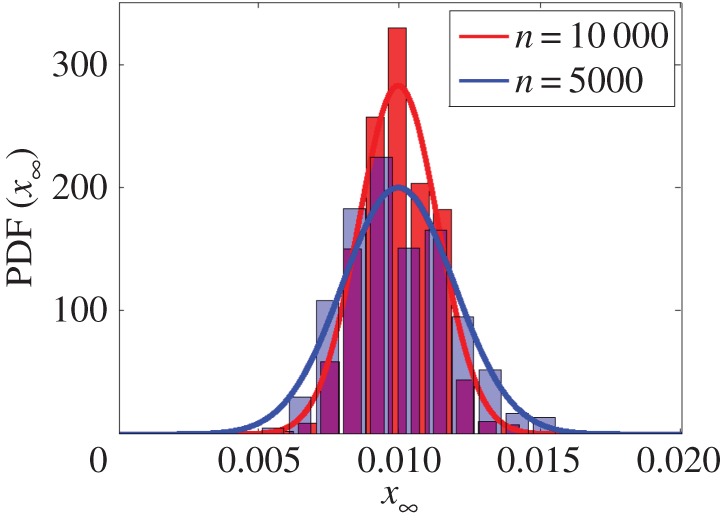
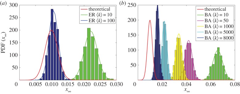
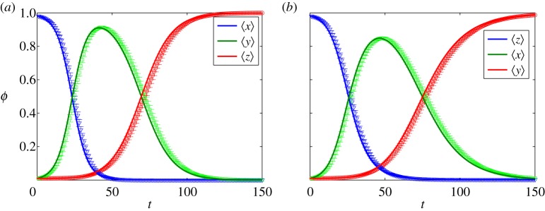
Rumour spreading is a ubiquitous phenomenon in social and technological networks. Traditional models consider that the rumour is propagated by pairwise interactions between spreaders and ignorants. Only spreaders are active and may become stiflers after contacting spreaders or stiflers. Here we propose a competition-like model in which spreaders try to transmit an information, while stiflers are also active and try to scotch it. We study the influence of transmission/scotching rates and initial conditions on the qualitative behaviour of the process. An analytical treatment based on the theory of convergence of density-dependent Markov chains is developed to analyse how the final proportion of ignorants behaves asymptotically in a finite homogeneously mixing population. We perform Monte Carlo simulations in random graphs and scale-free networks and verify that the results obtained for homogeneously mixing populations can be approximated for random graphs, but are not suitable for scale-free networks. Furthermore, regarding the process on a heterogeneous mixing population, we obtain a set of differential equations that describes the time evolution of the probability that an individual is in each state. Our model can also be applied for studying systems in which informed agents try to stop the rumour propagation, or for describing related susceptible-infected-recovered systems. In addition, our results can be considered to develop optimal information dissemination strategies and approaches to control rumour propagation.

Keywords: Monte Carlo simulation; asymptotic behaviour; density-dependent Markov Chain; epidemic model; rumour process; stochastic model.

Figure 1.

Time evolution of the rumour model (equation (3.2)) according to (a) the variation of the parameters α and λ for the fixed initial condition x₀=0.98,y₀= z₀=0.01 and (b) the variation of the initial condition for the fixed parameters α=0.05,λ=0.05.

Figure 2.

Fraction of ignorant individuals for the theoretical model, obtained by the numerical evaluation of the system of equations (3.2) for x₀=0.98, y₀=0.01 and z₀=0.01.

Figure 3.

Four different cases for the function f(x) given by equation (3.8). (a) ρ<x₀/z₀ and y₀>0, (b) ρ>x₀/z₀ and y₀>0, (c) ρ<x₀/z₀ and y₀=0 and (d) ρ>x₀/z₀ and y₀=0.

Figure 4.

Time evolution of the nodal probabilities considering our model for an ER network with n=10⁴ nodes and 〈k〉≈100. We consider the spreading rate λ=0.2 and stifling rate α=0.1. Each curve represents the probability that a node is in one of the three states (ignorant, spreader or stifler) and the colour represents the degree of the node i. The initial conditions are x₀=0.98, y₀=0.01 and z₀=0.01.

Figure 5.

Time evolution of the nodal probabilities considering our model for an BA network with n=10⁴ nodes and 〈k〉≈100. The spreading rate as λ=0.2, while the stifling rate is α=0.1. Each curve represents the probability that a node is in one of the three states (ignorant, spreader or stifler) and the colour represents the degree of the node i. The initial conditions are x₀=0.98, y₀=0.01 and z₀=0.01.

Figure 6.

Phase diagram of the final fraction of ignorants as a function of λ for α=0.5, $⟨x_{\mathrm{\infty }}⟩\times \mathrm{\lambda }$. The initial conditions are x₀=0.98, y₀=0.01 and z₀=0.01. All the networks have n=10³ nodes and 〈k〉≈10.

Figure 7.

Time evolution of the nodal probabilities considering the MT model in an ER network with n=10⁴ nodes and 〈k〉≈100. The spreading rate is λ=0.2 and the stifling rate is α=0.1. Each curve represents the probability that a node is in one of the three states (ignorant, spreader or stifler) and the colour represents the degree of the node i. The initial conditions are x₀=0.98, y₀=0.01 and z₀=0.01.

Figure 8.

Time evolution of the nodal probabilities considering the MT model in an BA network with n=10⁴ nodes and 〈k〉≈100. The spreading rate is λ=0.2 and the stifling rate is α=0.1. Each curve represents the probability that a node is in one of the three states (ignorant, spreader or stifler) and the colour represents the degree of the node i. The initial conditions are x₀=0.98, y₀=0.01 and z₀=0.01.

Figure 9.

Distribution of the fraction of ignorants obtained from 1000 simulations in a complete graph varying the number of nodes. The bars are obtained experimentally, while the fitted Gaussian are based on the theoretical values obtained from equations (3.2), (3.8) and (3.12).

Figure 10.

Distribution of the fraction of ignorants considering 1000 Monte Carlo simulations of the rumour scotching model in networks with n=10⁴ nodes generated from the (a) ER and (b) BA network models. The simulations consider λ=0.5, α=0.5 and initial conditions x₀=0.98, y₀=0.01 and z₀=0.01. Theoretical curves, obtained by equations (3.2), (3.8) and (3.12), are in red.

Figure 11.

Fraction of ignorants (given by colour intensities) according to the rates α and λ for different initial conditions considering ER, from (a–d), and BA network models, from (e–h). Networks with n=10⁴ and 〈k〉≈8 are considered. Every point is as an average over 50 simulations. (a) x₀=0.98, y₀=0.005 and z₀=0.015, (b) x₀=0.98, y₀=0.015 and z₀=0.005, (c) x₀=0.98, y₀=0.01 and z₀=0.01, (d) x₀=0.9, y₀=0.05 and z₀=0.05, (e) x₀=0.98, y₀=0.005 and z₀=0.015, (f) x₀=0.98, y₀=0.015 and z₀=0.005, (g) x₀=0.98, y₀=0.01 and z₀=0.01, and (h) x₀=0.9, y₀=0.05 and z₀=0.05.

Figure 12.

Comparison of the Monte Carlo simulations and the solution of the nodal time evolution differential equations, equations (4.5). The continuous curves are the numerical solution of the differential equations (4.5), while the symbols are the Monte Carlo simulations with its respective standard deviation. Every point is as an average over 50 simulations. In (a) an ER network while in (b) a BA network. Both with n=10⁴ nodes and 〈k〉≈100. Moreover, the initial conditions are x₀=0.98, y₀=0.01 and z₀=0.01.

References

-
- Castellano C, Fortunato S, Loreto V. 2009. Statistical physics of social dynamics. Rev. Mod. Phys. 81, 591–646. (doi:10.1103/RevModPhys.81.591) - DOI
- Lin W, Xiang L. 2014. Spatial epidemiology of networked metapopulation: an overview. Chin. Sci. Bull. 59, 3511–3522. (doi:10.1007/s11434-014-0499-8) - DOI - PMC - PubMed
- Agliari E, Burioni R, Cassi D, Neri FM. 2010. Word-of-mouth and dynamical inhomogeneous markets: efficiency measure and optimal sampling policies for the pre-launch stage. IMA J Manag. Math. 21, 67–83. (doi:10.1093/imaman/dpp003) - DOI
- Agliari E, Burioni R, Cassi D, Neri FM. 2006. Efficiency of information spreading in a population of diffusing agents. Phys. Rev. E 73, 046138 (doi:10.1103/PhysRevE.73.046138) - DOI - PubMed
- Keeling MJ, Eames KT. 2005. Networks and epidemic models. J. R. Soc. Interface 2, 295–307. (doi:10.1098/rsif.2005.0051) - DOI - PMC - PubMed
LinkOut - more resources
Full Text Sources
Other Literature Sources