Detection of Diffusion Heterogeneity in Single Particle Tracking Trajectories Using a Hidden Markov Model with Measurement Noise Propagation

Abstract

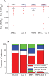
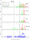
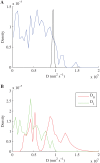
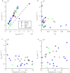
We develop a Bayesian analysis framework to detect heterogeneity in the diffusive behaviour of single particle trajectories on cells, implementing model selection to classify trajectories as either consistent with Brownian motion or with a two-state (diffusion coefficient) switching model. The incorporation of localisation accuracy is essential, as otherwise false detection of switching within a trajectory was observed and diffusion coefficient estimates were inflated. Since our analysis is on a single trajectory basis, we are able to examine heterogeneity between trajectories in a quantitative manner. Applying our method to the lymphocyte function-associated antigen 1 (LFA-1) receptor tagged with latex beads (4 s trajectories at 1000 frames s(-1)), both intra- and inter-trajectory heterogeneity were detected; 12-26% of trajectories display clear switching between diffusive states dependent on condition, whilst the inter-trajectory variability is highly structured with the diffusion coefficients being related by D1 = 0.68D0 - 1.5 × 10(4) nm2 s(-1), suggestive that on these time scales we are detecting switching due to a single process. Further, the inter-trajectory variability of the diffusion coefficient estimates (1.6 × 10(2) - 2.6 × 10(5) nm2 s(-1)) is very much larger than the measurement uncertainty within trajectories, suggesting that LFA-1 aggregation and cytoskeletal interactions are significantly affecting mobility, whilst the timescales of these processes are distinctly different giving rise to inter- and intra-trajectory variability. There is also an 'immobile' state (defined as D < 3.0 × 103 nm2 s-1) that is rarely involved in switching, immobility occurring with the highest frequency (47%) under T cell activation (phorbol-12-myristate-13-acetate (PMA) treatment) with enhanced cytoskeletal attachment (calpain inhibition). Such 'immobile' states frequently display slow linear drift, potentially reflecting binding to a dynamic actin cortex. Our methods allow significantly more information to be extracted from individual trajectories (ultimately limited by time resolution and time-series length), and allow statistical comparisons between trajectories thereby quantifying inter-trajectory heterogeneity. Such methods will be highly informative for the construction and fitting of molecule mobility models within membranes incorporating aggregation, binding to the cytoskeleton, or traversing membrane microdomains.

Fig 1. Fit of a two-state diffusion model without measurement noise to three stationary latex bead trajectories.

MCMC output from chains of 20000 MCMC steps with a 10000 step burn-in. (A-C) Inference of the hidden state z shown as the probability of being in the low diffusion state. (D-F) Posterior distributions for the two diffusion coefficients: D ₀ (red) and D ₁ (blue). See Methods for priors and initial conditions.

Fig 2. Model selection for one-state and two-state diffusion models on simulated stationary beads and stationary latex bead trajectories.

Blue bars: Bayes factors from model selection on simulated stationary beads (n = 240) with added Gaussian noise (σ ² = 41.09nm²). Single data points on axis: Bayes factors from model selection on stationary latex bead trajectories, both without (red asterisks) and with (green circles, σ ² = 41.09nm²) measurement noise incorporated into the inference algorithm. Priors, see Methods.

Fig 3. Fit of a two-state diffusion model with measurement noise to an LFA-1 trajectory (PMA+Cal-I treatment).

MCMC output (12 independent chains of 20000 MCMC steps with a 10000 step burn-in). (A) The posteriors for the two diffusion coefficients, (B) corresponding samples (12 chains plotted in the same colour) for D ₀ (red) and D ₁ (blue) including burn-in (dashed line). (C) Posteriors for the switching probabilities per frame, (D) corresponding samples (12 chains) for p ₀₁ (red) and p ₁₀ (blue) including burn-in (dashed line). (E) State inference shown as the probability of being in the low diffusion state. (F) Trajectory coloured by the probability of being in the low diffusion state. Colour scale represents π(z = 1∣X) from 0 (blue, high diffusion state) to 1 (green, low diffusion state). Colorbar length: 100nm. Priors, see Methods.

Fig 4. Model selection between approximate one-state and two-state diffusion models with measurement noise on LFA-1 trajectories.

(A) Box and whisker plot of log Bayes factors by treatment, trajectories with log Bayes factor outside 1.5 times IQR are plotted as outliers (red crosses). The thresholds ±3 (red lines) are shown. (B) Stacked bar plot showing proportions for each preferred model and trajectories which demonstrate fast switching between diffusive states. A log Bayes factor of ±3 ((A), red lines) is considered preference for the relevant model. MCMC runs comprise 12 parallel chains of 20000 steps with a 10000 step burn-in. Priors, see Methods.

Fig 5. Posterior estimates of diffusion coefficients for single LFA-1 trajectories.

(A-D) Pooled posterior samples of log_e D ₀ and log_e D ₁ for trajectories preferring the two-state diffusion model (fast switching, ${\widehat{p}}_{01}>0.1$ or ${\widehat{p}}_{10}>0.1$, trajectories removed). The posterior means for log_e D ₀ (red squares) and log_e D ₁ (green triangles), are also shown. Black line indicates value of σ ²/2Δt. Dashed line indicates threshold used to categorise immobile and mobile diffusion states. Treatments: (A) DMSO, two-state model preferred for 13 trajectories; (B) Cyto D, 3 trajectories; (C) PMA, 8 trajectories; (D) PMA+Cal-I, 6 trajectories. (E) Pooled log_e D estimates and posterior means (blue circles) over all treatments, for trajectories where one-state diffusion model was preferred (132 trajectories).

Fig 6. Pooled posterior distribution of diffusion coefficients for single LFA-1 trajectories.

(A) Pooled posterior samples of D for trajectories where one-state diffusion model was preferred, restricted to log_e D > 8 (99 trajectories). The posterior distribution from a single trajectory (black line, DMSO treatment) is also plotted, normalised to equal height. (B) Pooled posterior samples of D ₀ and D ₁ for trajectories where two-state diffusion model was preferred, restricted to log_e D ₁ > 8 (29 trajectories), with fast switching (${\widehat{p}}_{01}>0.1$ or ${\widehat{p}}_{10}>0.1$) trajectories removed. One data point with D ₀ > 2 × 10⁵ nm² s⁻¹ not shown.

Fig 7. Dependences of parameter estimates from two-state diffusion model.

(A-D) Scatter plots of posterior means for the two-state model with measurement noise, for trajectories where the approximate two-state diffusion model was preferred (fast switching, ${\widehat{p}}_{01}>0.1$ or ${\widehat{p}}_{10}>0.1$, trajectories removed). Treatments: DMSO, blue asterisks; Cyto D, red crosses; PMA, black circles; PMA+Cal-I, green triangles. In panel (A) the black solid line is a linear fit with two outlier trajectories removed, D ₁ = aD ₀ + b, a = 0.68, b = −1.5 × 10⁴ nm² s⁻¹; black dashed line is the double iterate, D ₁ = a(aD ₀ + b) + b.

Fig 8. Mean waiting times and example trajectories showing confinement for two-state diffusion model fit to LFA-1 trajectories.

(A) Mean waiting time in seconds ($1/\left(1000{\widehat{p}}_{01}\right)$ for z = 0 state, $1/(1000{\widehat{p}}_{10}$) for z = 1 state) for trajectories where approximate two-state diffusion model was preferred (fast switching, ${\widehat{p}}_{01}>0.1$ or ${\widehat{p}}_{10}>0.1$, trajectories removed). Treatments: DMSO, blue asterisks; Cyto D, red squares; PMA black circles; PMA+Cal-I, green triangles. Labels B-F correspond to example confinement state trajectories in B-F. (B) DMSO treatment (mean waiting time in z = 0 state 0.02s, in z = 1 state 0.04s) (C) PMA treatment (z = 0 state 0.32s, z = 1 state 0.16s) (D) PMA treatment (z = 0 state 0.09s, z = 1 state 0.12s) (E) PMA+Cal-I treatment (z = 0 state 1.48s, z = 1 state 0.39s) (F) DMSO treatment (z = 0 state 0.04s, z = 1 state 0.72s).

Fig 9. LFA-1 trajectories categorised as immobile (log_e D < 8 in the one-state model).

Trajectories are from different cells, with the first timepoints shifted to (0, 0). Treatments: DMSO (3 of 75 in immobile state), Cyto D (4 of 36 in immobile state), PMA (7 of 39 in immobile state), PMA+Cal-I D (20 of 46 in immobile state). Scalebars: 50nm.

Fig 10. Linear drifts in LFA-1 trajectories categorised as immobile (log_e D < 8 in the one-state model).

(A) Vertical displacements for two example trajectories. Blue line: DMSO treatment, ${\overline{v}}_y=117\text{nm}{\text{s}}^{-1}$; red line: PMA treatment, ${\overline{v}}_y=110\text{nm}{\text{s}}^{-1}$. (B-C) Displacements for a trajectory (PMA treatment) with a switch in drift direction. Estimated velocities: ${\overline{v}}_x=64\text{nm}{\text{s}}^{-1}$, ${\overline{v}}_y=80\text{nm}{\text{s}}^{-1}$, (average between 0 s and 2.25 s), ${\overline{v}}_y=-79\text{nm}{\text{s}}^{-1}$ (average between 2.25 s and 3.75 s), giving an average speed of 102 nm s⁻¹.

Fig 11. Comparison of parameter estimates for exact and approximate two-state diffusion models with measurement noise.

(A-D) Scatter plots of two-state parameter estimates for exact model against approximate model, for 30 trajectories preferring the approximate two-state model (fast-switching, ${\widehat{p}}_{01}>0.1$ or ${\widehat{p}}_{10}>0.1$ in the exact model, trajectories removed). Line of equality is shown as dashed. Treatments: DMSO (blue asterisks), Cyto D (red squares), PMA (black circles), PMA+Cal-I (green triangles).

Fig 12. Observed variation in the diffusion coefficient of LFA-1 in single particle tracking trajectories, with proposed mechanisms.

References

-
- Lingwood D, Simons K. Lipid rafts as a membrane-organizing principle. Science. 2010. January;327(5961):46–50. - PubMed
- Kusumi A, Nakada C, Ritchie K, Murase K, Suzuki K, Murakoshi H, et al. Paradigm shift of the plasma membrane concept from the two-dimensional continuum fluid to the partitioned fluid: high-speed single-molecule tracking of membrane molecules. Annual review of biophysics and biomolecular structure. 2005;34:351–378. 10.1146/annurev.biophys.34.040204.144637 - DOI - PubMed
Publication types
MeSH terms
Substances
LinkOut - more resources
Full Text Sources
Other Literature Sources