Topographic representations of object size and relationships with numerosity reveal generalized quantity processing in human parietal cortex

Abstract

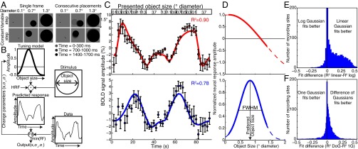
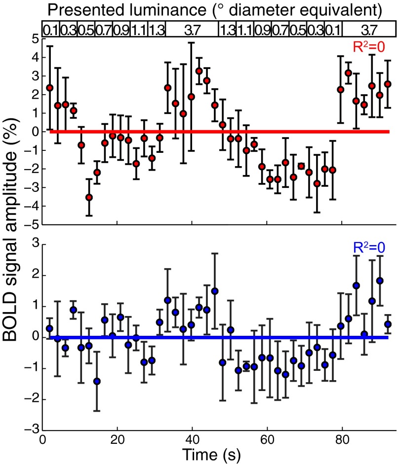
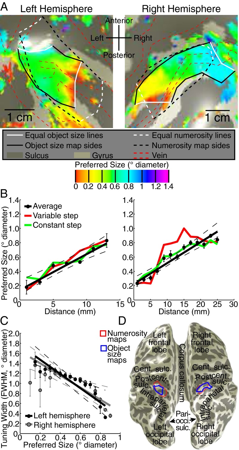
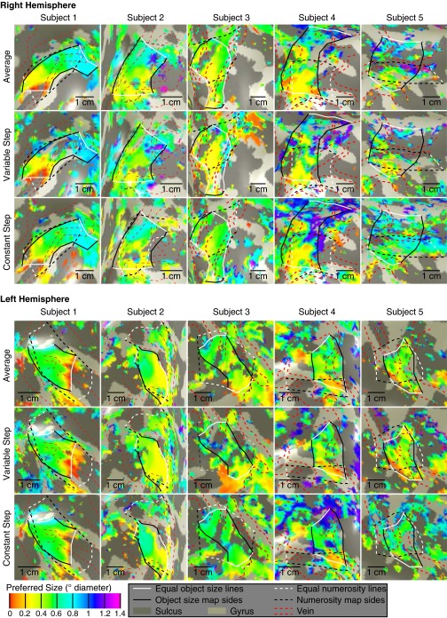
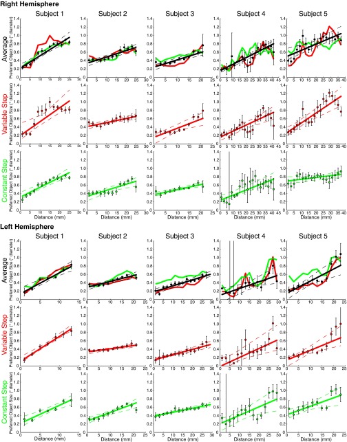
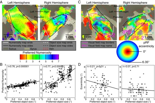
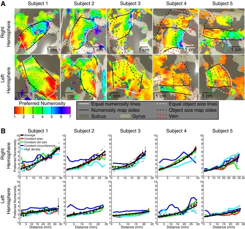
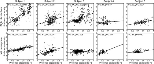
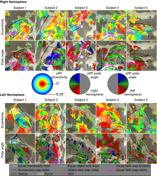
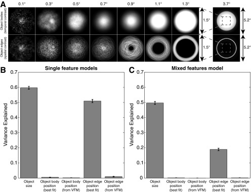
Humans and many animals analyze sensory information to estimate quantities that guide behavior and decisions. These quantities include numerosity (object number) and object size. Having recently demonstrated topographic maps of numerosity, we ask whether the brain also contains maps of object size. Using ultra-high-field (7T) functional MRI and population receptive field modeling, we describe tuned responses to visual object size in bilateral human posterior parietal cortex. Tuning follows linear Gaussian functions and shows surround suppression, and tuning width narrows with increasing preferred object size. Object size-tuned responses are organized in bilateral topographic maps, with similar cortical extents responding to large and small objects. These properties of object size tuning and map organization all differ from the numerosity representation, suggesting that object size and numerosity tuning result from distinct mechanisms. However, their maps largely overlap and object size preferences correlate with numerosity preferences, suggesting associated representations of these two quantities. Object size preferences here show no discernable relation to visual position preferences found in visuospatial receptive fields. As such, object size maps (much like numerosity maps) do not reflect sensory organ structure but instead emerge within the brain. We speculate that, as in sensory processing, optimization of cognitive processing using topographic maps may be a common organizing principle in association cortex. Interactions between object size and numerosity maps may associate cognitive representations of these related features, potentially allowing consideration of both quantities together when making decisions.

Keywords: high-field 7T fMRI; numerosity; object size; topographic maps.

Fig. 1.

Stimuli and pRF modeling. (A) Example stimuli. Objects were placed either randomly or pseudorandomly to lie entirely within 0.75° of fixation. Using purely random placements, smaller objects can take larger steps between consecutive placements (variable step condition). Therefore, we introduced a condition where objects always made steps of the same length in random directions (constant step condition). These two conditions gave very similar responses. (B) pRF modeling procedure (9, 11). A candidate neural tuning model describes a tuning function of an fMRI recording site, characterized by a preferred object size, tuning width, and suppressive surround width. Convolving the tuning model’s response amplitude with the time course of presented object sizes and the hemodynamic response function (HRF) predicts the fMRI response for this tuning model. For each recording site, we find the best-fitting tuning model parameters by minimizing the squared difference between the predicted fMRI response and the recorded data. (C) Two example fMRI time courses from sites in right posterior parietal cortex, about 2 cm apart, elicited by the presented object size time course (Top). Points represent mean response amplitudes; error bars represent the SE over repeated runs. In the Upper panel, the largest responses occur after presentation of small objects, whereas in the Lower panel the largest responses occur for larger objects, considering the hemodynamic response delay. The tuning model predictions (colored lines) capture over 75% of the variance (R²) in the time courses. BOLD, blood oxygen level-dependent. (D) The tuning models that explain the most variance in each time course. The model describes a linear Gaussian tuning function with a suppressive surround, characterized by two parameters: preferred object size and tuning width summarized by the function’s full width at half maximum (FWHM). Different tuning model parameters explain the different responses seen in C, capturing similar amounts of variance. Dashed lines show the continuation of tuning functions outside the presented object size range. (E) Linear one-Gaussian object size tuning models explain more response variance in most recording sites than logarithmic tuning models. Goodness of fit is evaluated by twofold cross-validation. Comparisons of difference of Gaussian tuning models give similar results. (F) Linear DoG object size tuning models explain more response variance in most recording sites than linear one-Gaussian models.

Fig. S1.

Stimuli varying in object size and numerosity over time yield different responses captured by different tuning models. (A) Two example fMRI time courses from sites in right posterior parietal cortex, about 2 cm apart, elicited by the presented object size sequence (Top). Points represent mean response amplitudes; error bars represent the SE over repeated runs. In the Upper panel, the largest response amplitude occurs after the presentation of small objects, whereas in the Lower panel the largest response occurs with larger objects, considering the hemodynamic response delay. The tuning model prediction captures much of the variance (R²) in the time courses, indicated by the colored lines. However, different tuning models capture different amounts of this variance. (B) Representation of the tuning models that best fit each time course. The best-fitting models describe linear Gaussian tuning functions with inhibitory surrounds. Tuning models describing other tuning functions perform less well, failing to capture features of the fMRI time courses in A. (C) fMRI time courses from the same two sites in A, elicited by the presented numerosity sequence (Top). Although these time courses are very different, the largest response amplitude in the Upper panel again occurs after the presentation of small numerosities, whereas in the Lower panel the largest response occurs with larger numerosities, considering the hemodynamic response delay. Again, tuning models capture much of the variance in the time courses, and different models capture different amounts of variance. (D) Representation of the tuning models that best fit each time course. The best-fitting models describe logarithmic Gaussian tuning functions. Tuning models describing linear tuning functions perform less well, failing to capture features of the fMRI time courses in C. Dashed lines show the continuation of tuning functions outside the presented object size range.

Fig. S2.

Responses to luminance-varying stimuli from the example recording sites shown in Fig. 1C and Fig. S1 (Upper and Lower panels here correspond to Upper and Lower panels of Fig. 1C and Fig. S1 A and C). To distinguish object size tuning from tuning to mean display luminance, we recorded responses to a stimulus where the mean luminance of the object size stimulus was distributed evenly across the largest object in the stimulus set, 1.3° diameter. During the long period that contained a 3.7°-diameter circle in the object size stimuli, the sequence also contained a 3.7°-diameter circle. Responses differed considerably from responses to stimuli of varying object size: They did not show tuned responses to a specific, low luminance, and response amplitudes increased when a larger circle was shown, which covered visual field positions that were not stimulated by the rest of the stimulus sequence.

Fig. 2.

Topographic representation of object size. (A) Object size preferences surrounding the previously described numerosity map (white and black dashed lines) (9) for data averaged from both stimulus conditions. Preferred object size changes gradually between lines of equal minimal and maximal preferred object size (white lines) in both hemispheres, forming topographic maps (black and white solid lines). Areas of low signal intensity, corresponding to pial veins (red dashed lines) (Fig. S3), were excluded from further analysis (21). (B) Object size preferences progress approximately linearly along the map. Recording sites were organized by their distances from the white lines in A. The two stimulus conditions are shown as colored lines joining condition-specific bin means. (C) Tuning width decreases as preferred object size increases. (D) Locations of object size and numerosity maps on an inflated cortical surface, relative to nearby major anatomical landmarks. Dashed boxes show the areas detailed in A. Cent., central; Pari-occi., parieto-occipital; Postcent, postcentral; Sulc., sulcus. In B and C, all dots represent the mean in each bin. Error bars represent SEs. All dashed lines represent 95% confidence intervals of the fit (solid line) to the bin means.

Fig. S3.

BOLD signal strength at each recording point in the average data across all object size and numerosity stimulus conditions, rendered on inflated cortical surfaces showing the same views as used in all other figures and supporting figures. Large draining veins on the pial surface and the superior sagittal sinus and its branches can be seen as areas of low signal strength. These are outlined with dashed lines, which correspond to the red dashed lines seen in other renderings of the cortical surface. Data from these areas are distorted, and the blood flow and oxygenation here result from neural activity elsewhere. Based on a subject-specific threshold of minimum signal strength in the average data, such recording points are excluded from analysis of preferred number and tuning width. The lines highlighting these areas are for illustration only. AU, arbitrary units.

Fig. S4.

Preferred object size varies across the cortical surface of right and left posterior parietal lobes in both stimulus conditions. Colors represent different object size preferences rendered on an inflated back view of the cortical surface. An area of clear topographic organization in all stimulus conditions is defined in black and white. The borders of this area representing minimum and maximum equal preferred object sizes are shown as white lines at the medial and lateral ends of the map. The posterior and anterior borders of this topographic representation are shown as black lines. Data are thresholded based on goodness of fit: In the average data, only recording points where R² is above 0.3 (P < 0.018 after false discovery rate correction) are shown; for all individual conditions the R² threshold is 0.25 (P < 0.031). Recording points where the model fits a preferred object size outside of the stimulus range are not shown. Dashed red lines outline distortions in the data caused by the presence of large veins on the pial surface (Fig. S3). This shows the areas around the previously described numerosity maps, whose borders are shown as black and white dashed lines.

Fig. S5.

Progression of preferred object size with distance along the map (shown in Fig. S4) for both stimulus conditions and the average data for each subject. Points represent the mean preferred object size in each distance bin, with error bars representing the SE. Solid lines are the best linear fit to the bin means. Dashed lines represent 95% confidence intervals determined by bootstrapping fits to the bin means. Object size preferences increase significantly across the map, at P = 0.01 or less in each hemisphere (permutation analysis).

Fig. S6.

Tuning width changes across the cortical surface with preferred object size. (A) Change in tuning width across the cortical surface for average data, showing the same views seen in Fig. S4, with the same threshold criteria. Tuning width decreases from the medial to the lateral ends of the map. (B) Tuning width shown as a function of preferred object size: Tuning width decreases as preferred object size increases. Recording points are binned based on preferred object size. Points represent the mean tuning width in each bin; error bars represent the SE. Solid lines are the best linear fit to the bins. Dashed lines represent 95% confidence intervals determined by bootstrapping fits to the bin means. Tuning widths decrease significantly with preferred object size, all at P = 0.007 or less in each hemisphere (permutation analysis).

Fig. 3.

Relationships between object size maps, numerosity maps, and visual field maps. (A) Numerosity preferences in the same areas as Fig. 2 form numerosity maps (solid black and white lines) that largely overlap with object size maps (dashed black and white lines). Left hemisphere numerosity maps are less clear than right, and represent a smaller numerosity range. Object size maps are similar bilaterally. (B) Among recording sites that lie in both maps, object size and numerosity preferences are correlated. The ratio of these preferences differs between hemispheres. (C) IPS visual field maps partially overlap with object size and numerosity maps. Object size- and numerosity-tuned responses were not limited to the central visual field positions where their stimuli were presented. Visual field map borders did not coincide with object size or numerosity map borders. (D) Among the fewer recording sites that lie in both visual field maps and object size or numerosity maps, neither object size nor numerosity preferences were correlated with pRF eccentricity or pRF size.

Fig. S7.

Maps of preferred numerosity. (A) Preferred numerosity varies across the cortical surface, in data averaged over all numerosity stimulus conditions. Topographic organization is clearer in the right hemisphere than in the left. Colors represent different preferred numerosities rendered on an inflated back view of the cortical surface, in the same area of cortex shown in Fig. S4. An area of clear topographic representation is defined in black and white. The borders of this area representing minimum and maximum equal preferred numerosities are shown as white lines at the medial and lateral ends of the map. The posterior and anterior borders of this topographic representation are shown as black lines. Data are thresholded based on goodness of fit: In the average data, only recording points where R² is above 0.3 (P < 0.007) are shown; for all individual conditions the R² threshold is 0.25 (P < 0.015). Recording points where the model fits a preferred numerosity outside of the stimulus range are not shown. Dashed red lines outline distortions in the data caused by the presence of large veins on the pial surface (Fig. S3). The object size maps described in Fig. S4 are shown as black and white dashed lines. (B) Progression of preferred numerosity with distance along the maps shown in A in the average data for each subject. Different stimulus conditions are represented as colored lines joining the condition-specific bin means. In the left hemisphere, the rate of change of preferred numerosity across the cortical surface is less than in the right hemisphere, as is the interquartile range of preferred numerosities present in the map. Map organization in the right hemisphere is also more consistent between conditions. Points represent the mean preferred numerosity in each distance bin, with error bars representing the SE. Solid lines are the fit to the bin means. These fit lines are straight in logarithmic space. Dashed lines represent 95% confidence intervals determined by bootstrapping fits to the binned points. For the average of all stimulus conditions, numerosity preferences increase significantly across the map, at P < 0.0001 in each hemisphere (permutation analysis).

Fig. S8.

Among recording sites that lie in both numerosity and object size maps, numerosity and object size preferences are correlated in both hemispheres. Although smaller numerosities are consistently found with smaller object sizes, the slope of this relationship differs between hemispheres. Significant correlation was absent in one hemisphere where the overlap of object size and numerosity maps covers little of the range of object size or numerosity preferences. r values are Pearson’s correlation coefficients. When calculating corresponding P values, the number of recording sites is adjusted to compensate for upsampling of data during transformation to cortical surface models. Lines represent the best-fitting linear relationship between object size and numerosity preferences.

Fig. S9.

Visual field map representations around the object size and numerosity maps, showing the same views seen in Figs. S4, S7, and S8. Borders between visual field maps are marked by purple lines. Dashed red lines show locations of veins, solid black and white lines show the borders of numerosity maps, and dashed black and white lines show the borders of object size maps, as in previous figures. Although visual field maps overlap with the object size numerosity maps, their borders do not correspond and there is no clear relationship between them. (Middle) Relationship between displayed color and preferred visual field position in visual field eccentricity and polar angle.

Fig. S10.

Among recording sites that lie in both object size maps and visual field maps, object size preferences and pRF properties of recording sites are not consistently correlated. (A) Preferred object size is not significantly correlated with pRF eccentricity. (B) Preferred object size is not significantly correlated with pRF size. (C) Preferred numerosity is not significantly correlated with pRF eccentricity. (D) Preferred numerosity is not significantly correlated with pRF size. r values are Pearson’s correlation coefficients, although Spearman’s rank correlation gives similar results. When calculating corresponding P values, the number of recording sites is adjusted to compensate for upsampling of data during transformation to cortical surface models. Lines represent the best-fitting linear relationship between object size preferences and pRF properties. Although some P values do reach significance at P < 0.05 in individual hemispheres, the directions of these correlations are not consistent between hemispheres, and only 1 of 40 remains significant after Bonferroni correction for multiple comparisons.

Fig. S11.

Distribution of visual field stimulation for different object sizes, and the potential predictive accuracy of retinotopic stimulation in explaining recorded responses. (A) Stimuli are designed to place object bodies randomly in the same stimulus area for all object sizes, minimizing links between particular visual field positions and particular object sizes. Furthermore, the largest object shown (3.7°) completely covers the area where other object sizes could be presented. This stimulates all these visual field positions but reduces response amplitudes. However, the positions of object edges are unavoidably linked to object size: Larger object sizes tend to have edges at higher eccentricities. Furthermore, the largest object has no edges in the central visual field, consistent with a decrease in response amplitude. Light intensities show positions where object bodies or edges are most likely to appear for a particular object size. (B) Response variance explained by separate models tuned to object size or visual field positions responding to object bodies or edges. Object size tuning predicts responses most closely, but tuned responses to object edge position can predict response well if allowed to choose any position tuning parameters. Here, pRF preferred positions are consistently at the visual field center, with position tuning widths (i.e., pRF sizes) increasing with preferred object size. Responses to conventional visual field mapping (VFM) stimuli, on the other hand, demonstrate that these recording sites prefer visual field positions outside the visual field center. If visual field position tuning properties are taken from VFM models, they predict responses poorly. (C) Response variance explained by the same response predictions when used as components of a single general linear model. Object size tuning continues to predict responses well, but any visual field position tuning captures little additional response variance. Error bars show 95% confidence intervals.

Fig. 4.

Object size tuning functions for a range of object size preferences, following average tuning parameters found across all hemispheres.

References

1. Cantlon JF, Brannon EM. Basic math in monkeys and college students. PLoS Biol. 2007;5(12):e328. - PMC - PubMed
1. Woodruff G, Premack D, Kennel K. Conservation of liquid and solid quantity by the chimpanzee. Science. 1978;202(4371):991–994. - PubMed
1. Dehaene S, Spelke E, Pinel P, Stanescu R, Tsivkin S. Sources of mathematical thinking: Behavioral and brain-imaging evidence. Science. 1999;284(5416):970–974. - PubMed
1. Burr D, Ross J. A visual sense of number. Curr Biol. 2008;18(6):425–428. - PubMed
1. Walsh V. A theory of magnitude: Common cortical metrics of time, space and quantity. Trends Cogn Sci. 2003;7(11):483–488. - PubMed
Publication types
LinkOut - more resources