Velocity-selective-inversion prepared arterial spin labeling

Abstract

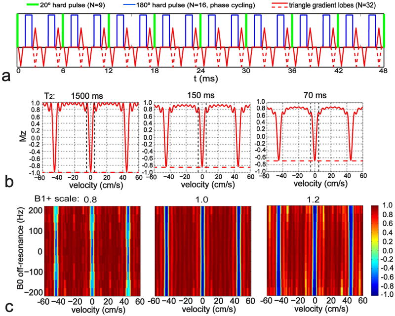
Purpose: To develop a Fourier-transform based velocity-selective inversion (FT-VSI) pulse train for velocity-selective arterial spin labeling (VSASL).

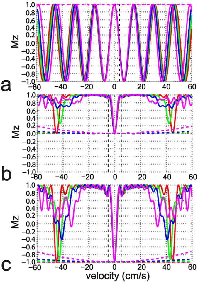
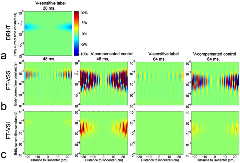
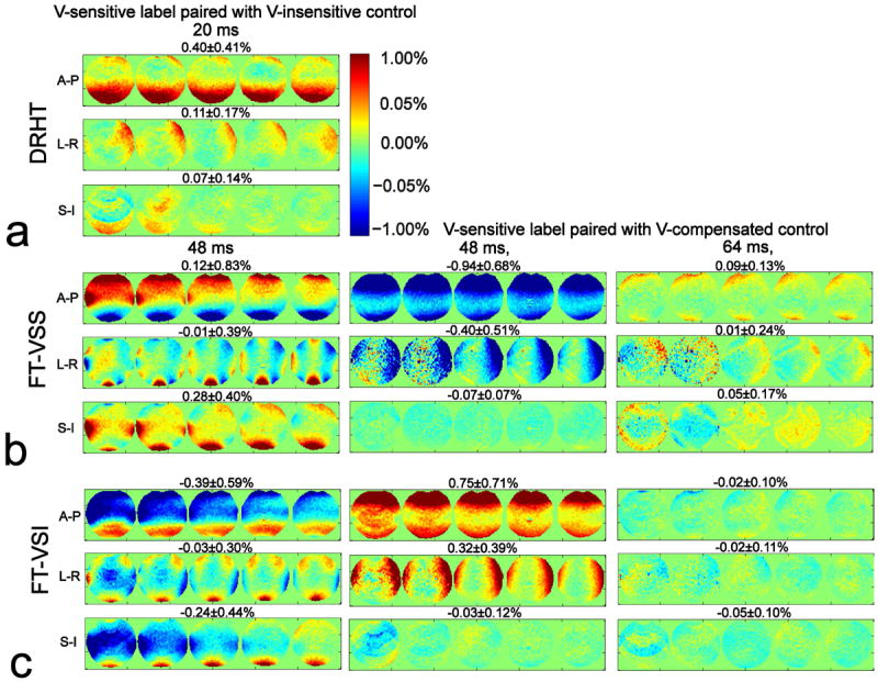
Methods: This new pulse contains paired and phase cycled refocusing pulses. Its sensitivities to B0/B1 inhomogeneity and gradient imperfections such as eddy currents were evaluated through simulation and phantom studies. Cerebral blood flow (CBF) quantification using FT-VSI prepared VSASL was compared with conventional VSASL and pseudocontinuous ASL (PCASL) at 3 Tesla.

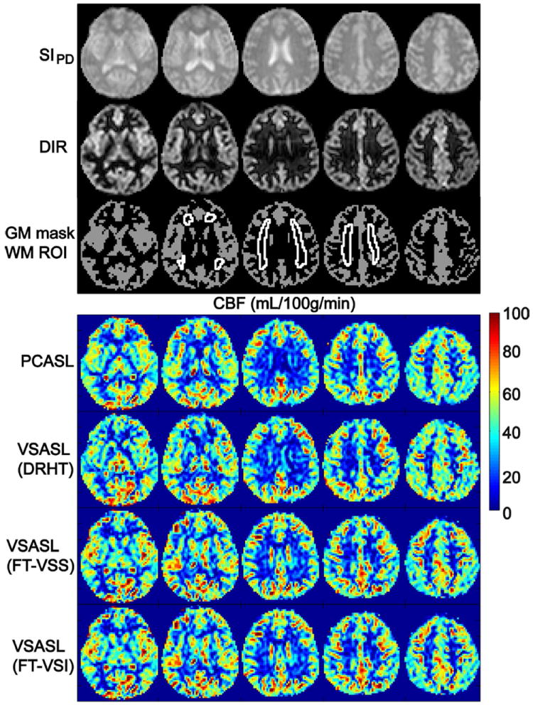
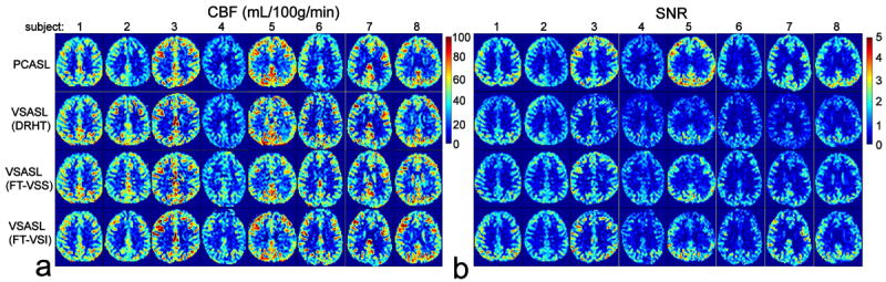
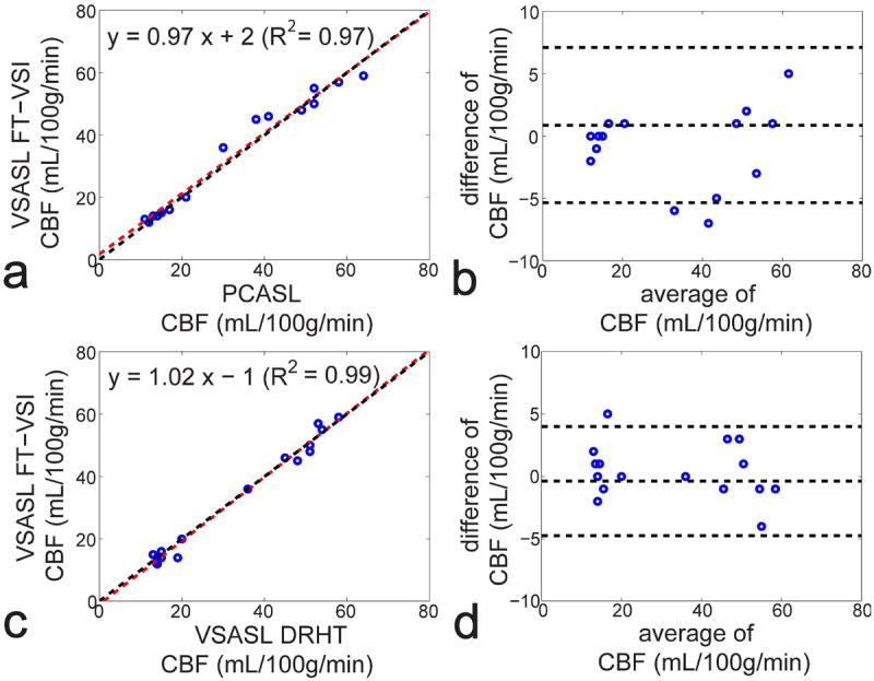
Results: Simulation and phantom results of the proposed FT-VSI pulse train demonstrated excellent robustness to B0/B1 field inhomogeneity and eddy currents. The estimated CBF of gray matter and white matter for the FT-VSI prepared VSASL, averaged among eight healthy volunteers, were 49.5 ± 7.5 mL/100 g/min and 14.8 ± 2.4 mL/100 g/min, respectively. Excellent correlation and agreement between the FT-VSI method and conventional VSASL and PCASL were found. The averaged signal-to-noise ratio (SNR) value in gray matter of the FT-VSI method was 39% higher than VSASL using conventional double refocused hyperbolic tangent pulses and 9% lower than PCASL.

Conclusion: A novel FT-VSI pulse train was demonstrated to be a suitable labeling module for VSASL with robustness of velocity-selective profile to B0/B1 field inhomogeneity and gradient imperfections. Compared with conventional VSASL, FT-VSI prepared VSASL produced consistent CBF maps with higher SNR values. Magn Reson Med 76:1136-1148, 2016. © 2015 Wiley Periodicals, Inc.

Keywords: B0 field inhomogeneity; B1 field inhomogeneity; Fourier transform; arterial spin labeling; cerebral blood flow; eddy current; k-space; velocity-selective inversion.

Figure 1

(a) Diagram of the FT-VSI pulse train with paired and phase-cycled refocusing pulses in each velocity encoding step, gradients with alternating polarity surrounding refocusing pulses for velocity-sensitized waveform (red solid lines) and uni-polar gradients for velocity-compensated waveform (red dashed lines for the polarity-switched gradient lobes). (b) The simulated Mz-Velocity responses of the pulse (a) with different T₂ relaxation effects: 1500 ms (CSF), 150 ms (arterial blood), and 70 ms (tissue). The vertical dashed lines indicate the inversion band (±4 cm/s). The horizontal dashed lines illustrate the universal inversion response of the FT-VSI pulse train for the control scan. (c) The simulated Mz-velocity responses of the labeling pulse (a) at different B0 conditions with representative B1+ scales of 0.8, 1.0, and 1.2.

Figure 2

The simulated Mz-velocity responses of the 20 ms DRHT (a), 64 ms FT-VSS (b), and 48 ms FT-VSI pulse trains (c) when encountering linear temporal velocity changes within 50 ms: constant velocities (red), from 95% to 105% (green), from 90% to 110% (blue), and from 80% to 120% (magenta). The dashed lines illustrate the responses for the control scans of these three pulse trains. No B0 or B1+ inhomogeneity or T₂ effects were included in this simulation.

Figure 3

The simulated differences of the Mz of static spins at different distances to isocenter, following the 20 ms DRHT (a), the 48 ms and 64 ms FT-VSS (b), the 48 ms and 64 ms FT-VSI pulse trains (c), in the presence of EC effects with different time constants, to the Mz at EC-free conditions. Velocity-sensitive (V-sensitive) labeling and velocity-compensated (V-compensated) control waveforms are both tested for each FT-VS configuration. B0/B1 inhomogeneity and T₂ effects were not taken into account.

Figure 4

Signal difference errors on a phantom for different VS label/control configurations, (a) 20 ms DRHT, (b) 48 ms and 64 ms FT-VSS, (c) 48 ms and 64 ms FT-VSI pulse trains, caused by gradient imperfections (such as EC) along different gradient orientations. Results for velocity-sensitive (V-sensitive) labeling paired with velocity-insensitive (V-insensitive) control are shown in the left column; the middle and right column display the results with velocity-compensated (V-compensated) controls. Error maps are normalized to SI_PD (percentage displayed). All acquired 5 slices are shown with the averaged error percentage (mean ± STD) displayed at the top of each row.

Figure 5

Representative data of all 5 slices acquired from subject 8: images of the SI_PD; image of gray matter only from the DIR sequence, the segmented GM mask and WM ROI, quantified CBF maps using PCASL and VSASL scans employing DRHT, FT-VSS, and FT-VSI labeling techniques, respectively.

Figure 6

Examples of the estimated CBF maps (a) and SNR images (b) of 8 subjects (only one slice shown), using PCASL and VSASL scans employing DRHT, FT-VSS, and FT-VSI labeling techniques, respectively.

Figure 7

Correlation (a,c) and agreement plots (b,d) of the averaged individual CBF values of both GM and WM (open circles) measured by FT-VSI prepared VSASL with PCASL (a,b) and DRHT-prepared VSASL (c,d), respectively. For the correlation plots (a,c), red dashed lines are the linear regression curves with the fitted equations shown at the top of the figures. The black dashed lines show the unity line y = x. For the agreement plots (b,d), the difference of the two methods are plotted against the mean (Bland-Altman plot), with the middle of the three horizontal dashed lines indicating the mean difference of all subjects, and the top and bottom dashed lines indicating the mean difference ± two times of the standard deviation of their differences.

References

1. Dai W, Garcia D, de Bazelaire C, Alsop DC. Continuous flow-driven inversion for arterial spin labeling using pulsed radio frequency and gradient fields. Magn Reson Med. 2008;60(6):1488–1497. - PMC - PubMed
1. Dai W, Robson PM, Shankaranarayanan A, Alsop DC. Reduced resolution transit delay prescan for quantitative continuous arterial spin labeling perfusion imaging. Magn Reson Med. 2012;67(5):1252–1265. - PMC - PubMed
1. Qin Q, Huang AJ, Hua J, Desmond JE, Stevens RD, van Zijl PC. Three-dimensional whole-brain perfusion quantification using pseudo-continuous arterial spin labeling MRI at multiple post-labeling delays: accounting for both arterial transit time and impulse response function. NMR Biomed. 2014;27:116–128. - PMC - PubMed
1. Gunther M, Bock M, Schad LR. Arterial spin labeling in combination with a look-locker sampling strategy: inflow turbo-sampling EPI-FAIR (ITS-FAIR) Magn Reson Med. 2001;46(5):974–984. - PubMed
1. Qiu M, Paul Maguire R, Arora J, Planeta-Wilson B, Weinzimmer D, Wang J, Wang Y, Kim H, Rajeevan N, Huang Y, Carson RE, Constable RT. Arterial transit time effects in pulsed arterial spin labeling CBF mapping: insight from a PET and MR study in normal human subjects. Magn Reson Med. 2010;63(2):374–384. - PMC - PubMed
Publication types