Robust and efficient parameter estimation in dynamic models of biological systems

Abstract

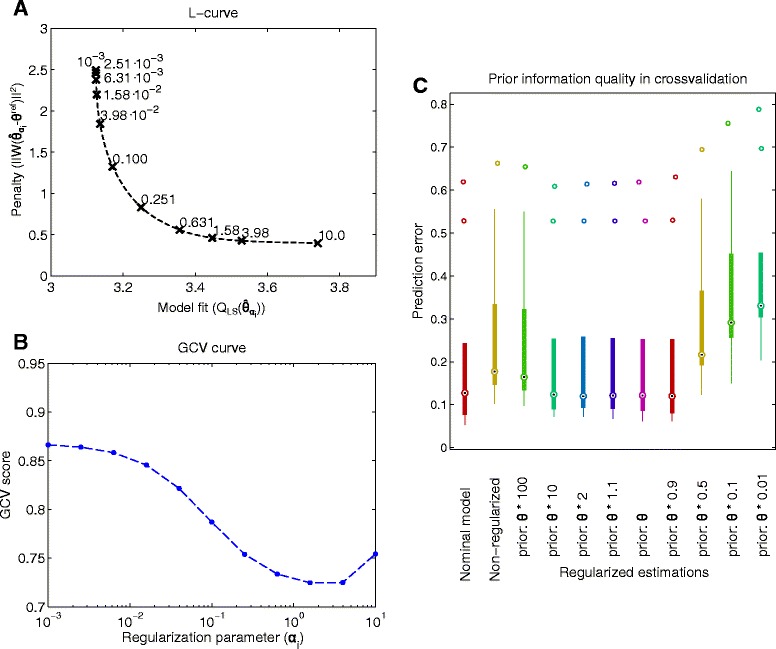
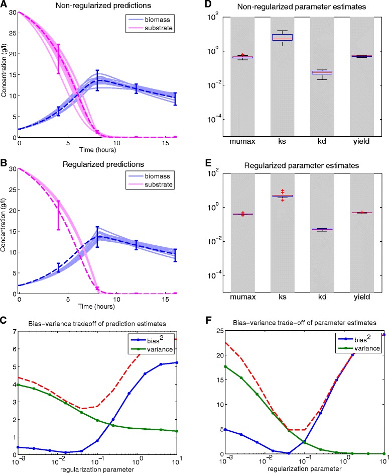
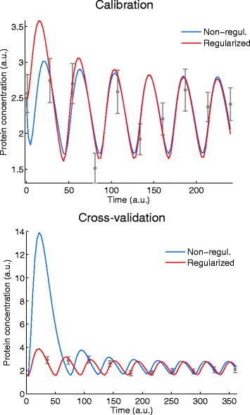
Background: Dynamic modelling provides a systematic framework to understand function in biological systems. Parameter estimation in nonlinear dynamic models remains a very challenging inverse problem due to its nonconvexity and ill-conditioning. Associated issues like overfitting and local solutions are usually not properly addressed in the systems biology literature despite their importance. Here we present a method for robust and efficient parameter estimation which uses two main strategies to surmount the aforementioned difficulties: (i) efficient global optimization to deal with nonconvexity, and (ii) proper regularization methods to handle ill-conditioning. In the case of regularization, we present a detailed critical comparison of methods and guidelines for properly tuning them. Further, we show how regularized estimations ensure the best trade-offs between bias and variance, reducing overfitting, and allowing the incorporation of prior knowledge in a systematic way.

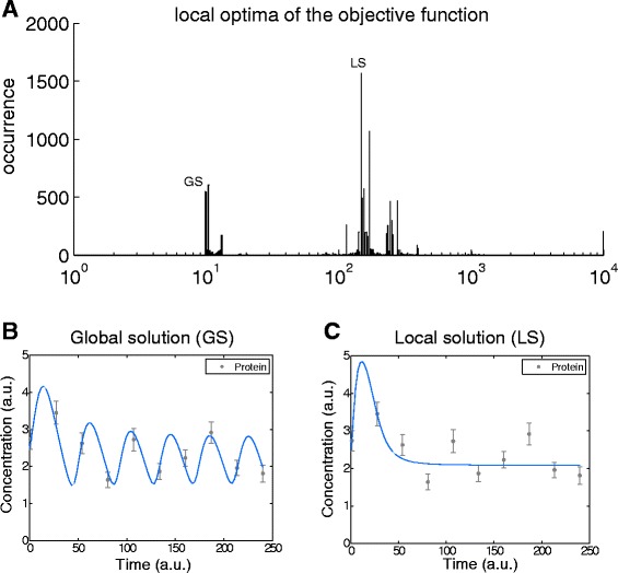
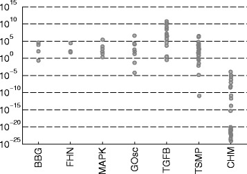
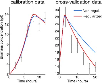
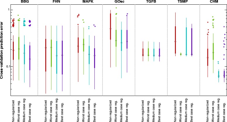
Results: We illustrate the performance of the presented method with seven case studies of different nature and increasing complexity, considering several scenarios of data availability, measurement noise and prior knowledge. We show how our method ensures improved estimations with faster and more stable convergence. We also show how the calibrated models are more generalizable. Finally, we give a set of simple guidelines to apply this strategy to a wide variety of calibration problems.

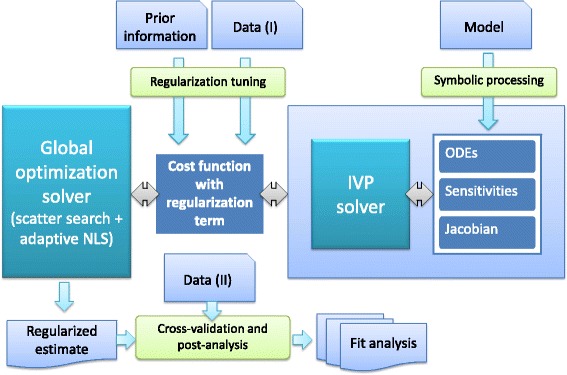
Conclusions: Here we provide a parameter estimation strategy which combines efficient global optimization with a regularization scheme. This method is able to calibrate dynamic models in an efficient and robust way, effectively fighting overfitting and allowing the incorporation of prior information.

Fig. 1

Architecture of the method: in the pre-processing phase, sensitivity equations and Jacobians (both of the residuals and of the differential equations) are derived via symbolic manipulation, generating C code which is then linked to the initial value problem (IVP) solver, CVODES. The regularization scheme is selected according to the quality of the prior knowledge, and tuned following the procedure described in section “Tuning the regularization and prior knowledge”. Finally, global optimization with eSS2 is used to find the regularized estimate of the parameters. The resulting calibrated model can then be further evaluated using cross-validation, followed by additional post-regression and goodness-of-fit analysis

Fig. 2

Local optima of the objective function corresponding to the Goodwin’s oscillator case study (GOsc). Figure a shows the distribution of the final objective function values of 10,000 runs of local solver NL2SOL from randomly chosen initial points based on Latin hypercube sampling. The distribution of the local optima shows that only 6 % of the runs finished in the close vicinity of the global optima (minimum objective function value: 9.8903). Figure b shows the fit corresponding to the global optima (global solution – GS). Figure c depicts the fit corresponding to the most frequently achieved local minima (local solution – LS, objective function value: 148.25). Note the qualitatively wrong behaviour of this fit, i.e. the lack of oscillations in the predictions

Fig. 3

Distributions of local optima for all case studies. Each case study was solved by the AMS method and the observed frequency of the local minima is reported here. Note that the objective function values (Q _LS) are scaled by the global optimum QLSGO for each case study, and the resulting ratio is reported in logarithmic scale. The height of the first bin at 0 represents the frequency of finding the vicinity of the global solution

Fig. 4

Comparison of convergence curves of selected optimization methods. The convergence curve shows the value of the objective function versus the computation time during the minimization (model calibration). Results are given for simple multi- start (SMS), advanced multi-start (AMS) and enhanced scatter search methods (eSS2a and eSS2b; see description in main text). Results are shown for two case studies: (a) GOsc and (b) TSMP

Fig. 5

Tuning the regularization method for BBG case study. Figure a shows the trade-off between the two terms of the regularized objective function, i.e. model fit and the regularization penalty, for a set of regularization parameters (values shown close to symbols). A larger regularization parameter results in worse fit to the calibration data, small regularization parameter results in a larger penalty. Figure b compares the candidates based on the generalized cross-validation scores. A larger score indicates worse model prediction for cross-validation data. The curve has the minimum at 1.58. Figure c shows the normalized root mean square prediction error of calibrated model for 10 sets of cross-validation data and regularizations considering different quality of the prior information (initial guess of the parameters). For a wide range of priors (initial guesses based on the reference parameter vector) the regularized estimation gives a good cross-validation error. Small priors exhibit worse predictions

Fig. 6

Bias-variance trade-off for the BBG case study. Figures a and b illustrate the nominal trajectory (dashed line) and the range of perturbed measurements together with predictions of calibrated models (continuous lines) without and with regularization, respectively. The distribution of the regularized predictions (in b) are narrower than in the non- regularized one (in a), but are slightly biased from the nominal trajectory. Figure c depicts the squared bias and the variance of these model predictions as a function of the regularization parameter. The mean square error (dashed line) has a minimum at 0.08. Figure d, e and f shows the results for the estimated parameters: with regularization the estimated parameters are less sensitive to perturbations in the data

Fig. 7

Eigenvalues of the approximated Hessian matrix for each case study. Eigenvalues are related to the identifiability of the model parameters: a large spread indicates lack of identifiability of some parameters from the given dataset

Fig. 8

Calibration and cross-validation results for the BBG case study. Left figure shows calibration data fitted with non-regularized and regularized estimations (non-regularized, $Q_{\text{LS}}\left(\widehat{\theta }\right)=3.68$ and regularized $Q_{\text{LS}}\left({\widehat{\theta }}_{\alpha }\right)=4.09$). Right figure shows cross-validation data with the predictions from the non-regularized and regularized estimations. The regularized model shows a slightly worse fit to the calibration data but much better agreement with the cross-validation data. I.e. regularization results in a more generalizable model

Fig. 9

Calibration and cross-validation results for the GOsc case study. Left figure shows fits to calibration data, right figure shows agreement of predictions for cross-validation data. The non-regularized and the regularized fits show some differences in the first two oscillations, although at the measurement times the predictions are almost identical. In cross-validation, the non-regularized model shows a heavy overshoot at early times

Fig. 10

Prediction errors distribution for each case study. Prediction errors (box-plots of normalized root mean square error in log-scale) of the calibrated models with and without regularization are shown for each case study. These distributions were obtained by calibrating the models to multiple sets of calibration data (as explained in section “Ill-conditioning, cross-validation and overfitting”) and cross-validating them on multiple cross-validation data sets. Most cases show the trend that better prior knowledge results in smaller cross-validation errors, i.e. regularized models are more generalizable

References

1. Mogilner A, Wollman R, Marshall WF. Quantitative modeling in cell biology: what is it good for? Dev Cell. 2006;11(3):279–87. doi: 10.1016/j.devcel.2006.08.004. - DOI - PubMed
1. Epstein JM. Why model? J Artif Soc Social Simul. 2008;11(4):12.
1. Wolkenhauer O. Why model? Front Physiol. 2014;5:21. doi: 10.3389/fphys.2014.00021. - DOI - PMC - PubMed
1. Lander AD. The edges of understanding. BMC Biol. 2010;8(1):40. doi: 10.1186/1741-7007-8-40. - DOI - PMC - PubMed
1. Wolkenhauer O. Systems biology: the reincarnation of systems theory applied in biology? Brief Bioinform. 2001;2(3):258–70. doi: 10.1093/bib/2.3.258. - DOI - PubMed
Publication types
LinkOut - more resources