Ultrasonic tracking of shear waves using a particle filter

Abstract

Purpose: This paper discusses an application of particle filtering for estimating shear wave velocity in tissue using ultrasound elastography data. Shear wave velocity estimates are of significant clinical value as they help differentiate stiffer areas from softer areas which is an indicator of potential pathology.

Methods: Radio-frequency ultrasound echo signals are used for tracking axial displacements and obtaining the time-to-peak displacement at different lateral locations. These time-to-peak data are usually very noisy and cannot be used directly for computing velocity. In this paper, the denoising problem is tackled using a hidden Markov model with the hidden states being the unknown (noiseless) time-to-peak values. A particle filter is then used for smoothing out the time-to-peak curve to obtain a fit that is optimal in a minimum mean squared error sense.

Results: Simulation results from synthetic data and finite element modeling suggest that the particle filter provides lower mean squared reconstruction error with smaller variance as compared to standard filtering methods, while preserving sharp boundary detail. Results from phantom experiments show that the shear wave velocity estimates in the stiff regions of the phantoms were within 20% of those obtained from a commercial ultrasound scanner and agree with estimates obtained using a standard method using least-squares fit. Estimates of area obtained from the particle filtered shear wave velocity maps were within 10% of those obtained from B-mode ultrasound images.

Conclusions: The particle filtering approach can be used for producing visually appealing SWV reconstructions by effectively delineating various areas of the phantom with good image quality properties comparable to existing techniques.

FIG. 1.

A pictorial representation of the relationships between various random variables (input, hidden states, and output) of the hidden Markov model is shown here. Every hidden state M_n has two components, and the observed values Y_n are obtained after addition of i.i.d. zero mean Gaussian noise to the first component. The second component is the local slope value S_n which obeys a Markov structure. The slope stays constant with a probability p and changes to a new uniformly randomly chosen value with a probability 1 − p; the uniform random variable X_n acts as an input to the model.

FIG. 2.

A cross-sectional view (not to scale) of the two phantoms used for experimental validation is shown in (a). Both phantoms consist of a stiff ellipsoidal inclusion embedded in a softer background material. The stiff region mimics the presence of completely ablated tissue, whereas the softer background simulates unablated tissue. An irregularly shaped partially ablated region of intermediate stiffness is present on one side of the inclusion. A block diagram of the data acquisition system is shown in (b). The needle is vibrated in a single pulse motion using an actuator operated in synchronization with the ultrasound scanner. RF echo data are acquired from a linear array transducer.

FIG. 3.

Frame-to-frame displacements are obtained from the RF echo data and TTP is estimated from displacement vs time profiles for each pixel in the imaging plane. Displacement profiles for six different pixels using data from Phantom-1 are shown in (a). The six displacement plots correspond to pixels located at lateral distances from 0 to 1.8 cm in increments of 0.3 cm and at a depth of 3 cm. A zoomed section of the displacement profiles is shown in (b). This noise causes uncertainty in exact values of TTP which appears as noise in the TTP plot shown in (c). Two particle filter fits with p = 0.85 and p = 0.95 are also shown overlaid on the noisy TTP. Note that the smaller value of p results in more “jumps” in the final fit as seen from the SWV estimates. The TTP values and frame numbers are related via the imaging frame rate.

FIG. 4.

MSE of estimated slope values from three different noise filtering methods applied to randomly generated piecewise linear data. Simulated piecewise linear data were filtered using three different filtering algorithms (pf = particle filter, poly = 4th order polynomial, movav = moving average 10 point window, sg2 = Savitzky–Golay quadratic with 10 point span, sg3 = Savitzky–Golay cubic with 15 point span, raw = no filtering). Local slope values were estimated by finite differencing. MSE from 50 independent simulated data vectors is presented in this figure. The particle filter provided the lowest mean MSE. (a) p = 0.85, (b) p = 0.90, and (c) p = 0.95.

FIG. 5.

SWV maps reconstructed from data obtained from the finite element simulation model are shown here. The top row shows images reconstructed using a particle filter with parameters (p, σ²) = (0.98, 0.25) (pf), moving average 10 point window (movav), Savitzky–Golay quadratic with 15 point span (sg2), and Savitzky–Golay cubic with 20 point span (sg3), respectively, from left to right. The bottom row shows SWV values along a horizontal line at a constant depth of 3 cm. True SWV profiles from the finite element model are shown with dotted lines.

FIG. 6.

A finite element simulation model was used to export frame-to-frame displacements which were processed using various algorithms to estimate SWV. Mean squared reconstruction error in the SWV maps produced from the finite element simulation model is shown here, where the SWV from the finite element model was used as ground truth. (pf = particle filter, movav = moving average 10 point window, sg2 = Savitzky–Golay quadratic with 15 point span, sg3 = Savitzky–Golay cubic with 20 point span, raw = no filtering.)

FIG. 7.

The ideal SWV image from the finite element model is shown in (a). The ground truth SWV values are 4.28 and 1.28 m/s in the inclusion and the background, respectively. A representative TTP plot along a line at a depth of 3 cm to the right of the needle is shown in (b). The SWV image shown in (c) is generated by processing these TTP curves at all depths using the particle filter. Since the SWV values are obtained using a Bayesian model, the posterior density can be used to produce a standard deviation image that provides feedback about the reliability of the SWV estimates. The standard deviation image in (d) is calculated using the square root of the quantity in Eq. (10) for each pixel in the SWV image.

FIG. 8.

ROIs and inclusion boundaries used for Phantom-1 are shown. Boundary used for B-mode area estimation is shown in (a). Boundaries for area estimation and ROIs used for calculating various statistics on the SWV maps are shown in (b), (c), and (d).

FIG. 9.

ROIs and inclusion boundaries used for Phantom-2 are shown. Boundary used for B-mode area estimation is shown in (a). Boundaries for area estimation and ROIs used for calculating various statistics on the SWV maps are shown in (b), (c), and (d).

FIG. 10.

SWV maps obtained using the clinical software interface of the Supersonic Imagine Aixplorer scanner using SSI are shown. Results from Phantom-1 and Phantom-2 are shown in (a) and (b), respectively. Reconstructions using the particle filtering algorithm are shown again on the same SWV scale for comparison in (c) and (d).

FIG. 11.

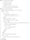
Details of the particle filter algorithm in pseudocode adapted from Algorithm 6 in the paper by Arulampalam et al. (Ref. 19) and Section V of Doucet et al. (Ref. 24).

FIG. 12.

Resampling algorithm used within the particle filter algorithm shown in Fig. 11.

FIG. 13.

Backward smoothing routine used in the particle filter algorithm shown in Fig. 11.

References

1. Sarvazyan A., Rudenko O., Swanson S., Fowlkes J. B., and Emelianov S., “Shear wave elasticity imaging: A new ultrasonic technology of medical diagnostics,” Ultrasound Med. Biol. 24(9), 1419–1435 (1998).10.1016/S0301-5629(98)00110-0 - DOI - PubMed
1. Palmeri M., Wang M., Dahl J., Frinkley K., and Nightingale K., “Quantifying hepatic shear modulus in vivo using acoustic radiation force,” Ultrasound Med. Biol. 34(4), 546–558 (2008).10.1016/j.ultrasmedbio.2007.10.009 - DOI - PMC - PubMed
1. Sandrin L., Tanter M., Catheline S., and Fink M., “Shear modulus imaging with 2-D transient elastography,” IEEE Trans. Ultrason., Ferroelectr., Freq. Control 49(4), 426–435 (2002).10.1109/58.996560 - DOI - PubMed
1. Sandrin L., Tanter M., Gennisson J., Catheline S., and Fink M., “Shear elasticity probe for soft tissues with 1-D transient elastography,” IEEE Trans. Ultrason., Ferroelectr., Freq. Control 49(4), 436–446 (2002).10.1109/58.996561 - DOI - PubMed
1. Bharat S. and Varghese T., “Radiofrequency electrode vibration-induced shear wave imaging for tissue modulus estimation: A simulation study (L),” J. Acoust. Soc. Am. 128(4), 1582–1585 (2010).10.1121/1.3466880 - DOI - PMC - PubMed
Publication types