Remote control of self-assembled microswimmers

Abstract

Physics governing the locomotion of microorganisms and other microsystems is dominated by viscous damping. An effective swimming strategy involves the non-reciprocal and periodic deformations of the considered body. Here, we show that a magnetocapillary-driven self-assembly, composed of three soft ferromagnetic beads, is able to swim along a liquid-air interface when powered by an external magnetic field. More importantly, we demonstrate that trajectories can be fully controlled, opening ways to explore low Reynolds number swimming. This magnetocapillary system spontaneously forms by self-assembly, allowing miniaturization and other possible applications such as cargo transport or solvent flows.

Figure 1. Self-assembled magnetocapillary swimmer.

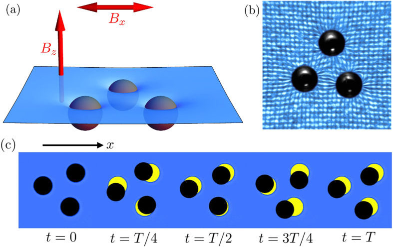
(a) Sketch of the magnetocapillary system. Soft ferromagnetic particles are self-assembling at the water-air interface in a Petri dish. A vertical and constant magnetic field B_z is applied through the system. An oscillating horizontal field B_x excites the motion of the self-assembled structure. (b) A top view of the interface emphasizes the self-assembly of D = 500μm beads in a vertical field: capillary attraction is counterbalanced by dipole-dipole repulsion. The deformation of the liquid-air interface is evidenced by placing an array of pixels underneath the Petri dish. (c) Five snapshots of the beads over one period T of the forcing oscillation. The traces of the initial positions are drawn in yellow for emphasizing the motion of the structure. One should notice the rotational oscillation of the structure during the period.

Figure 2. Selection of swimming modes.

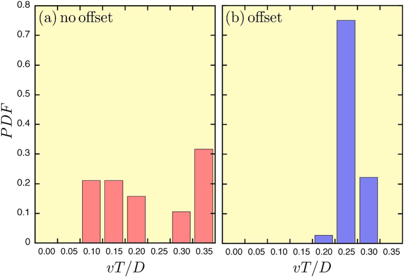
Probability Distribution Function (PDF) of normalized speeds obtained in similar experimental conditions: β_x = 7.5 G and f = 0.5 Hz, but (a) without an offset, (b) with a constant offset B_x0 = 0.75 G. The plots are obtained from 55 independent realizations.

Figure 3. Swimming speeds.

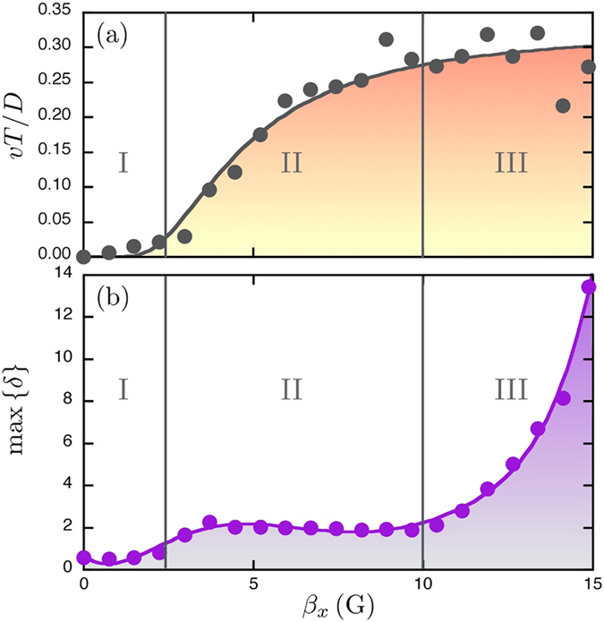
(a) Average speed of the self-assembled system as a function of the amplitude of oscillations, when the offset is B_x0 = 0.75 G and f = 0.5 Hz. The velocity is seen to increase and saturates around 0.3 D/T. The curve is a guide for the eye. (b) The maximum standard deviation δ of the angles from the regular triangle as a function of the amplitude β_x. The curve is a guide for the eye. Please note the large differences obtained near the collapse (β_x ≈ 15 G). Three regimes (I, II and III) are indicated and are discussed in the main text.

Figure 4. Full control of swimming trajectories.

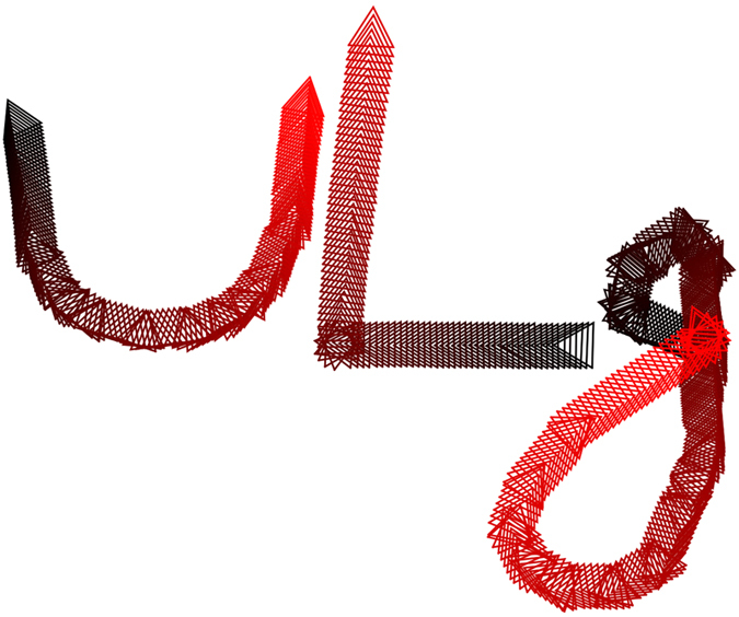
The remote control of a microswimmer, by adjusting the horizontal field orientation , allows us to follow various paths such as U-turn, corner and loops. Laid next to one another, the three letters of “ULg” are then obtained. Bead centers are tracked for drawing the triangles at each period, emphasizing the orientation of the structure. The colors indicate the time evolution of each trajectory from dark to red.

Figure 5. Model for non-reciprocal motion.

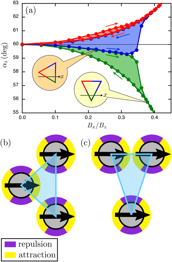
(a) Internal angles given by the model as a function of the increasing or decreasing horizontal magnetic interaction (see arrows). Angles α_i are colored after being sorted from the smallest to the largest. Two triangles are illustrated using the same color code in order to evidence the orientation of the structure at two specific situations: and ∇ states. (b) Sketch of the platy-isosceles () configuration. Arrows indicate the horizontal components of the dipoles. Colors indicate whether a pair of dipoles attract or repel compared to zero horizontal field, which depends on their relative orientation. (c) Sketch of the lepto-isosceles (∇) configuration.

Figure 6. Non-reciprocal motion in the experiment.

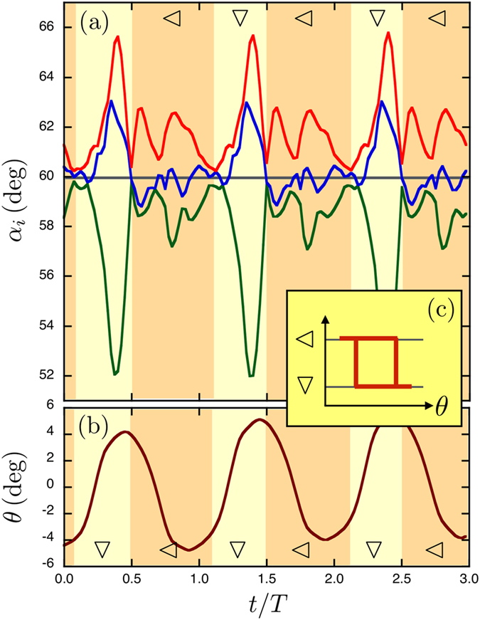
(a) Three periods T of the angles α_i with the same color code as in Fig. 5(a), using our experimental data. One observes that the blue curve oscillates between the red and green ones in each period. The system switches periodically between and ∇ isosceles. (b) The angle θ of the whole structure during three periods. Oscillations are seen evidencing the successive switches. (c) This sketch shows the isosceles states as a function of θ forming a loop at each cycle, i.e. a non-reciprocal motion.