Effect of trial-to-trial variability on optimal event-related fMRI design: Implications for Beta-series correlation and multi-voxel pattern analysis

Abstract

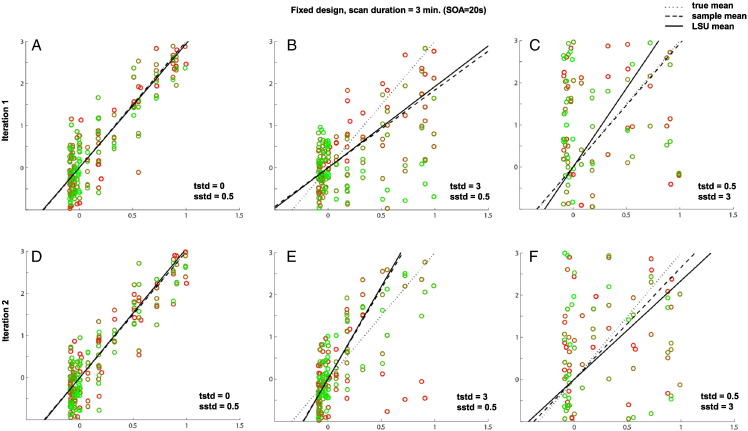
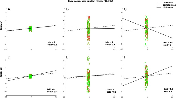
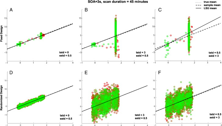
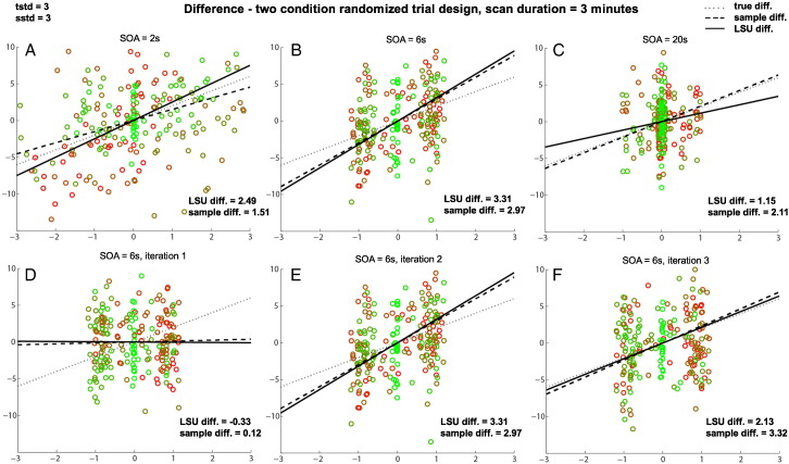
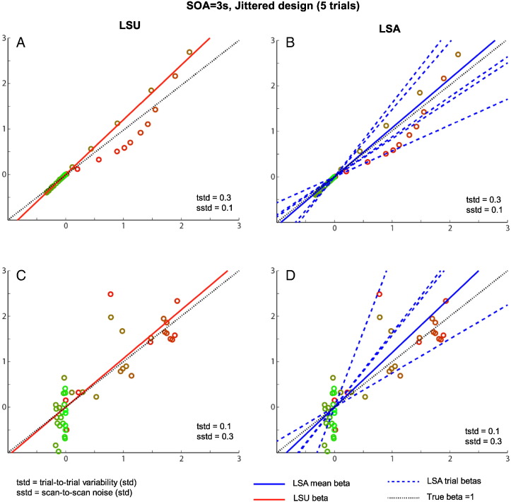
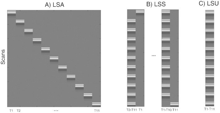
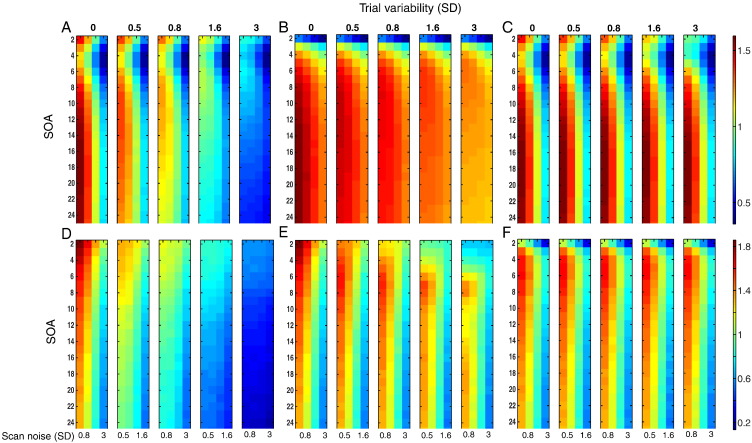
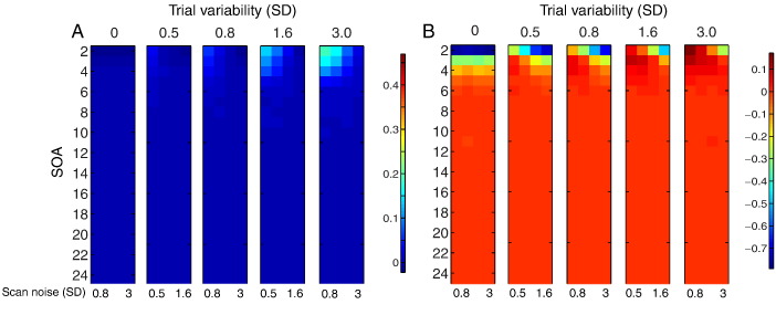
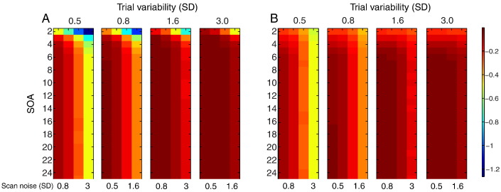
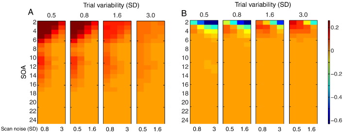
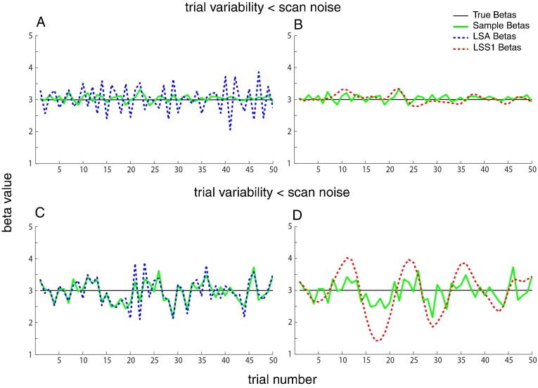
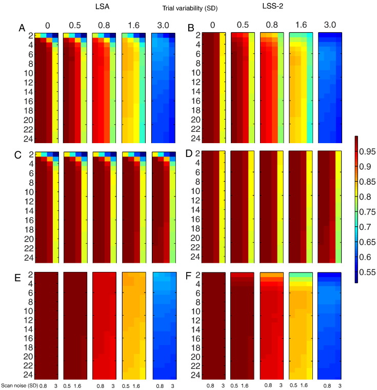
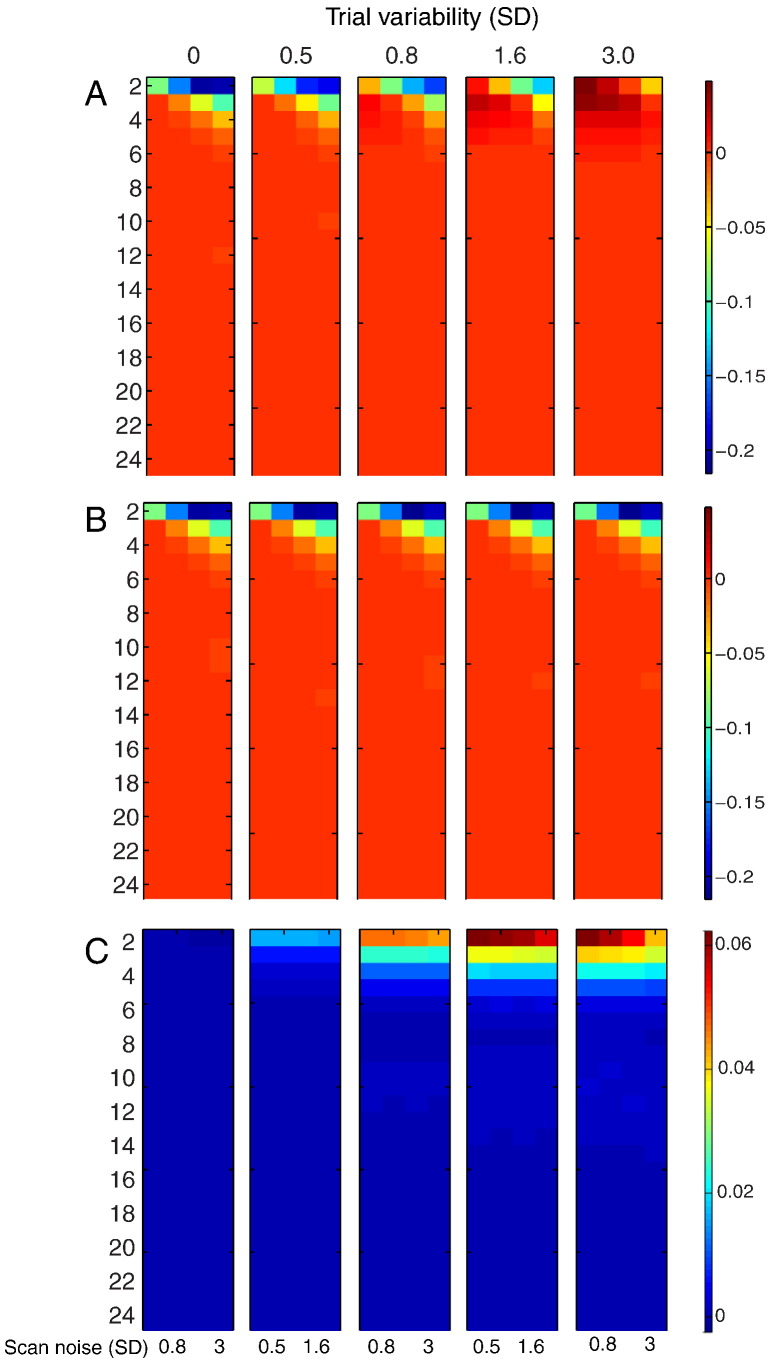
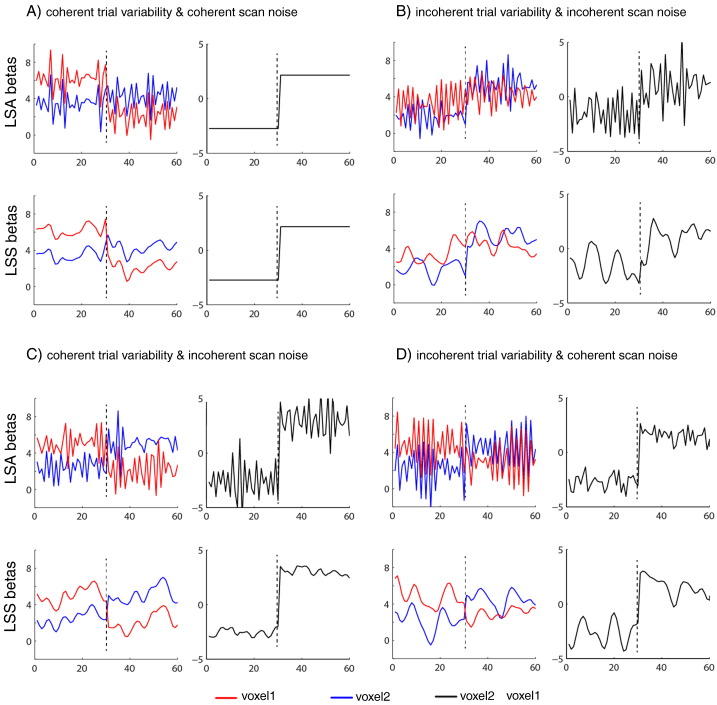
Functional magnetic resonance imaging (fMRI) studies typically employ rapid, event-related designs for behavioral reasons and for reasons associated with statistical efficiency. Efficiency is calculated from the precision of the parameters (Betas) estimated from a General Linear Model (GLM) in which trial onsets are convolved with a Hemodynamic Response Function (HRF). However, previous calculations of efficiency have ignored likely variability in the neural response from trial to trial, for example due to attentional fluctuations, or different stimuli across trials. Here we compare three GLMs in their efficiency for estimating average and individual Betas across trials as a function of trial variability, scan noise and Stimulus Onset Asynchrony (SOA): "Least Squares All" (LSA), "Least Squares Separate" (LSS) and "Least Squares Unitary" (LSU). Estimation of responses to individual trials in particular is important for both functional connectivity using "Beta-series correlation" and "multi-voxel pattern analysis" (MVPA). Our simulations show that the ratio of trial-to-trial variability to scan noise impacts both the optimal SOA and optimal GLM, especially for short SOAs<5s: LSA is better when this ratio is high, whereas LSS and LSU are better when the ratio is low. For MVPA, the consistency across voxels of trial variability and of scan noise is also critical. These findings not only have important implications for design of experiments using Beta-series regression and MVPA, but also statistical parametric mapping studies that seek only efficient estimation of the mean response across trials.

Keywords: Bold variability; General Linear Model; Least squares all; Least squares separate; MVPA; Trial based correlations; fMRI design.

Supplementary Fig. 1

Effects of trial variability and scan noise on efficiency of estimating the mean of single trial-type using LSU when SOA = 20 s. tstd = trial beta standard deviation, sstd = scan noise standard deviation. The scatter plots show simulated BOLD activity (y-axis) against LSU's regressor (x-axis) for a 3 min session sampled at TR = 1 s, after removing the transients in the first and last 32 s. The black solid line is the linear least-squares fit, whose slope corresponds to the LSU parameter estimate; the slope of the dashed line corresponds to the sample mean; the slope of the dotted line corresponds to the true (population) mean (here equal to 3). The more closely the dots fall to the best-fit line, the more accurate the estimation of the slope of that line. The closer the solid line to the dotted line, the more precise the estimate of the population mean (i.e., PPM in main paper). Note that there are the same number of dots (scans) in each panel, which are bunched into vertical columns, where the number of columns corresponds to the SOA and the number of dots per column corresponds to the number of trials. The dot colors change smoothly from green to red in proportion to the proximity to the beginning and the end of the session (i.e., dots with similar hue are close together in time). In comparison to the first column (with only a small amount of scan noise), it can be seen that the LSU estimate (solid line) deviates more from the true mean (dotted line) as the trial-variability (middle column) or scan noise (bottom column) increases, as in Fig. 2B of the paper. The top and bottom panels indicate two simulations with different samples of trial variability and scan noise. The difference between PPM and PSM can be seen by comparing top and bottom panels. In panels B and E, for example, though the LSU estimate (solid line) differs from the true mean (dotted line), it closely tracks the sample mean (dashed line). This is why the PSM does not decease with increasing trial variability in Fig. 2C of the paper.

Supplementary Fig. 2

Effects of trial variability and scan noise on efficiency of estimating the mean of single trial-type using LSU when SOA = 3 s. See legend of Supplementary Fig. 1 for more details. Effects of trial variability and scan noise on efficiency of estimating the mean of single trial-type using LSU when SOA = 3 s. See legend of Supplementary Fig. 1 for more details. When SOA is short, the spread of points along the x-axis reduces compared to Supplementary Fig. 1 (where SOA = 20 s), and this reduced range prevents precise estimate of the slope of the best-fitting line, which is why PPM generally decreases as SOA decreases in Fig. 2B of main paper (without the influence of transients; cf Supplementary Fig. 3). When SOA is short, the spread of points along the x-axis reduces compared to Supplementary Fig. 1 (where SOA = 20 s), and this reduced range prevents precise estimate of the slope of the best-fitting line, which is why PPM generally decreases as SOA decreases in Fig. 2B of main paper (without the influence of transients; cf Supplementary Fig. 3). A more subtle point is that, when trial-variability is high and scan noise low (Panels B and E), the LSU estimate (solid line) can be closer to the true mean (dotted line), on average across simulations, than when the SOA is longer (cf. Panels B and E of Supplementary Fig. 1). This is because a shorter SOA entails more trials in total, i.e., a greater number of columns, and better “anchoring” the best-fitting line. This explains why the optimal SOA for PPM decreases as trial-variability increases in Fig. 2B of main paper. Note that the sample mean is independent of the number of trials, so the optimal SOA does not change this way for PSM in Fig. 2C of main paper. A more subtle point is that, when trial-variability is high and scan noise low (Panels B and E), the LSU estimate (solid line) can be closer to the true mean (dotted line), on average across simulations, than when the SOA is longer (cf. Panels B and E of Supplementary Fig. 1). This is because a shorter SOA entails more trials in total, i.e., a greater number of columns, and better “anchoring” the best-fitting line. This explains why the optimal SOA for PPM decreases as trial-variability increases in Fig. 2B of main paper. Note that the sample mean is independent of the number of trials, so the optimal SOA does not change this way for PSM in Fig. 2C of main paper.

Supplementary Fig. 3

Effects of transients on efficiency of estimating a single trial-type (top row) and efficiency for two randomly-intermixed trial-types (bottom row) when SOA = 3 s. See legend of Supplementary Fig. 1 for more details. Effects of transients on efficiency of estimating a single trial-type (top row) and efficiency for two randomly-intermixed trial-types (bottom row) when SOA = 3 s. See legend of Supplementary Fig. 1 for more details. Transients at the start and end of the session, which correspond to the second, smaller cluster of points near x = 0 in the top row, help to stabilize the slope of the regression line, relative to Supplementary Fig. 2, even though only representing a small fraction of the total number of scans (the session is now 45 min long). This explains the second peak at short SOA in Fig. 2A (but not Fig. 2B) of main paper. Transients at the start and end of the session, which correspond to the second, smaller cluster of points near x = 0 in the top row, help to stabilize the slope of the regression line, relative to Supplementary Fig. 2, even though only representing a small fraction of the total number of scans (the session is now 45 min long). This explains the second peak at short SOA in Fig. 2A (but not Fig. 2B) of main paper. The SOA in the lower panels is a randomized intermixed design of two trial-types, but one of which has a mean and standard deviation of 0 (equivalent to a “null event” in the terminology of Josephs and Henson, 1999). This jittering dramatically increases efficiency (cf. Panel D with Supplementary Figs. 1A and 2A), consistent with standard efficiency theory, which explains the optimally short SOA in Fig. 2D of the main paper. Note also that transients also have little effect in such designs. The SOA in the lower panels is a randomized intermixed design of two trial-types, but one of which has a mean and standard deviation of 0 (equivalent to a “null event” in the terminology of Josephs and Henson, 1999). This jittering dramatically increases efficiency (cf. Panel D with Supplementary Figs. 1A and 2A), consistent with standard efficiency theory, which explains the optimally short SOA in Fig. 2D of the main paper. Note also that transients also have little effect in such designs.

Supplementary Fig. 4

Effects of SOA on PSM for difference between two randomly-intermixed trial-types for three different SOAs (top row) and three different iterations when SOA = 6 s (bottom row) when trial variability plus scan noise are high. See legend of Supplementary Fig. 1 for more details. Effects of SOA on PSM for difference between two randomly-intermixed trial-types for three different SOAs (top row) and three different iterations when SOA = 6 s (bottom row) when trial variability plus scan noise are high. See legend of Supplementary Fig. 1 for more details. In this case, one is interested in the best estimate of the difference in slopes for the two trial-types, regardless of whether the slope of each trial-type is itself estimated efficiently. If the scan noise is low (not shown), the difference between trial-types can be estimated best for shortest SOAs (like in Supplementary Fig. 3), even though the slopes of individual trial-types are estimated better when SOA is longer (explaining the difference in optimal SOA for Fig. 2B versus 2E in main paper, and consistent with different optimal SOAs for [1 − 1] and [1 1] contrasts in Josephs and Henson, 1999). In this case, one is interested in the best estimate of the difference in slopes for the two trial-types, regardless of whether the slope of each trial-type is itself estimated efficiently. If the scan noise is low (not shown), the difference between trial-types can be estimated best for shortest SOAs (like in Supplementary Fig. 3), even though the slopes of individual trial-types are estimated better when SOA is longer (explaining the difference in optimal SOA for Fig. 2B versus 2E in main paper, and consistent with different optimal SOAs for [1 − 1] and [1 1] contrasts in Josephs and Henson, 1999). However, unlike the jittered SOA shown in bottom row of Supplementary Fig. 3, both trial-types now have non-zero trial variabilities. This means that when the scan noise is high (as shown here), it becomes difficult to distinguish differences between trial-types from random variations in scan noise. This makes estimation of the true difference in slopes worse, as shown in Fig. 2B in main paper. Estimation of the difference in sample means, however, is optimal for intermediate SOAs (like SOA = 6 s here). The reason for this is that at these SOAs, the scans (points) fall into two clumps near the ends of the best-fit line, which serve to better “anchor” that line. This is shown in the bottom row, with three different random samples of data at SOA = 6 s, where the LSU estimate tracks the sample difference, even though both vary considerably from the population difference (owing to the high trial variability). This explains the peak around SOA = 6 s with high trial variability for PSM in Fig. 2E of the main paper, but not for PPM in Fig. 2D. However, unlike the jittered SOA shown in bottom row of Supplementary Fig. 3, both trial-types now have non-zero trial variabilities. This means that when the scan noise is high (as shown here), it becomes difficult to distinguish differences between trial-types from random variations in scan noise. This makes estimation of the true difference in slopes worse, as shown in Fig. 2B in main paper. Estimation of the difference in sample means, however, is optimal for intermediate SOAs (like SOA = 6 s here). The reason for this is that at these SOAs, the scans (points) fall into two clumps near the ends of the best-fit line, which serve to better “anchor” that line. This is shown in the bottom row, with three different random samples of data at SOA = 6 s, where the LSU estimate tracks the sample difference, even though both vary considerably from the population difference (owing to the high trial variability). This explains the peak around SOA = 6 s with high trial variability for PSM in Fig. 2E of the main paper, but not for PPM in Fig. 2D.

Supplementary Fig. 5

Comparison between LSU (left panels) and LSA (right panels) for a short SOA (3 s) jittered design of only 5 trials, with either low (top row) or higher (bottom row) scan noise. See legend of Supplementary Fig. 1 for more details, though note that true (population) beta is now 1, for illustration purposes. Comparison between LSU (left panels) and LSA (right panels) for a short SOA (3 s) jittered design of only 5 trials, with either low (top row) or higher (bottom row) scan noise. See legend of Supplementary Fig. 1 for more details, though note that true (population) beta is now 1, for illustration purposes. When trial-to-trial variability is higher than the scan noise, as in the upper row, the LSU model in Panel A cannot account for all the variability from trial-to-trial, and some trials (brown colored points) have a greater effect on the best-fitting slope than other trials (red points). The LSA model, on the other hand, can effectively fit a different line to each trial (dashed blue lines), as shown in Panel B, producing a better overall fit (and less affected by more extreme points). When averaging the slopes (Betas) from each trial, one can obtain a more precise estimate of the population mean, as in Fig. 2F of the main paper. However, when scan noise is higher than the trial-to-trial variability, as in the bottom row, LSA's extra flexibility (higher degrees of freedom) in Panel D means that some of its individual trial estimates fit the scan noise instead. This results in LSA over-fitting the data, and hence its estimate of the population mean (averaging across trials) now becomes less precise than for the more constrained LSU fit in Panel A. Together, this explains why the relative advantage of LSU vs LSA (at short SOA) depends on the ratio of trial variability to scan noise, as shown in Fig. 3 of the main paper.

Fig. 1

Design matrices for (A) LSA (Least Squares-All), (B) LSS (Least Squares-Separate) and (C) LSU (Least Squares-Unitary). T(number) = Trial number.

Fig. 2

Efficiency for estimating mean of a single trial-type (top panels) or the mean difference between two trial-types (bottom panels) as a function of SOA and scan noise for each degree of trial variability. Panels A–C show results for a single-trial-type LSU model, using A) precision of population mean (PPM), B) PPM without transients, and C) precision of sample mean (PSM). Panels D–E show results for difference between two randomly intermixed trial-types, using D) PPM and E) PSM. Panel F shows corresponding PSM results but using LSA model (LSS gives similar results to LSU). The top number on each subplot represents the level of trial-to-trial variability, y-axes are the SOA ranges and x-axes are scan noise levels. The color map is scaled to base-10 logarithm, with more efficient estimates in hotter colors, and is the same for panels A–C (shown right top) and D–F (shown right bottom).

Fig. 3

Log of ratio of PPM for LSA relative to LSU models for (A) estimating mean of a single trial-type, or (B) the mean difference between two randomly intermixed trial-types, as a function of SOA and scan noise for each degree of trial variability. The color maps are scaled to base-10 logarithm. See Fig. 2 legend for more details.

Fig. 4

Log of precision of Sample Correlation (PSC) for two randomly intermixed trial-types for LSA (A) and LSS-1 (B). See Fig. 2 legend for more details.

Fig. 5

Log of ratio of PSC in Fig. 4 for (A) LSS-2 relative to LSS-1 and (B) LSA relative to LSS-2. See Fig. 2 legend for more details.

Fig. 6

Example of sequence of parameter estimates (${\widehat{\beta }}_j$) for 50 trials of one stimulus class with SOA of 2 s (true population mean B = 3) when trial variability (SD = 0.3) is greater than scan noise (SD = 0.1; top row) or trial variability (SD = 0.1) is less than scan noise (SD = 0.3; bottom row), from LSA (left panels, in blue) and LSS (right panels, in red). Individual trial responses β_j are shown in green (identical in the left and right plots).

Fig. 7

SVM classification performance for LSA (panels A + C + E) and LSS-2 (panels B + D + F) for (A) incoherent trial variability and incoherent scan noise (panels A + B), coherent trial variability and incoherent scan noise (panels C + D), and incoherent trial variability and coherent scan noise (panels E + F). Note color bar is not log-transformed (raw accuracy, where 0.5 is chance and 1.0 is perfect). Note that coherent and incoherent cases are equivalent when trial variability is zero (but LSA and LSS are not equivalent even when trial variability is zero). See Fig. 2 legend for more details.

Fig. 8

Log of ratio of LSA relative to LSS-2 SVM classification performance in Fig. 7 for (A) incoherent trial variability and incoherent scan noise, (B) coherent trial variability and incoherent scan noise and (C) incoherent trial variability and coherent scan noise. Note that coherent and incoherent cases are equivalent when trial variability is zero. See Fig. 2 legend for more details.

Fig. 9

Panels A, B, C and D show different variations of coherency of trial-to-trial variability and scan noise across two voxels (SOA = 2 s and both trial SD and scan SD = 0.5). In each Panel, plots on left show parameters/estimates for 30 trials of each of two trial-types: true parameters (β_j) for trials 1–30 are 5 and 3 for voxel 1 and voxel 2 respectively, while true parameters (β_j) for trials 31–60 are 3 and 5 for voxel 1 and voxel 2 respectively. Plots on right show difference between voxels for each trial (which determines CP). Upper plots in each panel show corresponding parameter estimates (${\widehat{\beta }}_j$) from LSA model; lower plots show estimates from LSS-2 model.

References

1. Baum S.H., Beauchamp M.S. Greater BOLD variability in older compared with younger adults during audiovisual speech perception. PLoS ONE. 2014;9 - PMC - PubMed
1. Becker R., Reinacher M., Freyer F., Villringer A., Ritter P. How ongoing neuronal oscillations account for evoked fMRI variability. J. Neurosci. 2011;31:11016–11027. - PMC - PubMed
1. Birn R.M. The behavioral significance of spontaneous fluctuations in brain activity. Neuron. 2007;56:8–9. - PubMed
1. Brignell C.J., Browne W.J., Dryden I.L., Francis S.T. Mixed Effect Modelling of Single Trial Variability in Ultra-high Field fMRI. 2015. ArXiv preprint, ArXiv: 1501.05763
1. Chawla D., Rees G., Friston K.J. The physiological basis of attentional modulation in extrastriate visual areas. Nat. Neurosci. 1999;2:671–676. - PubMed