Seasonal fluxes of carbonyl sulfide in a midlatitude forest

Abstract

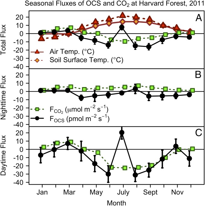
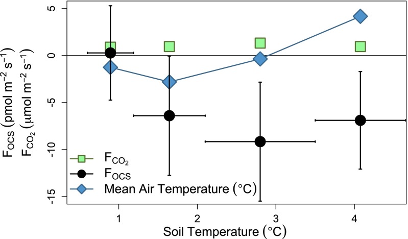
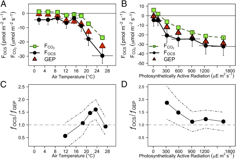
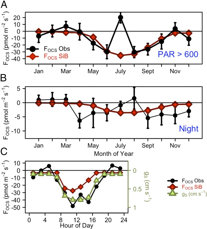
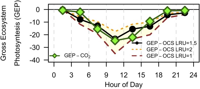
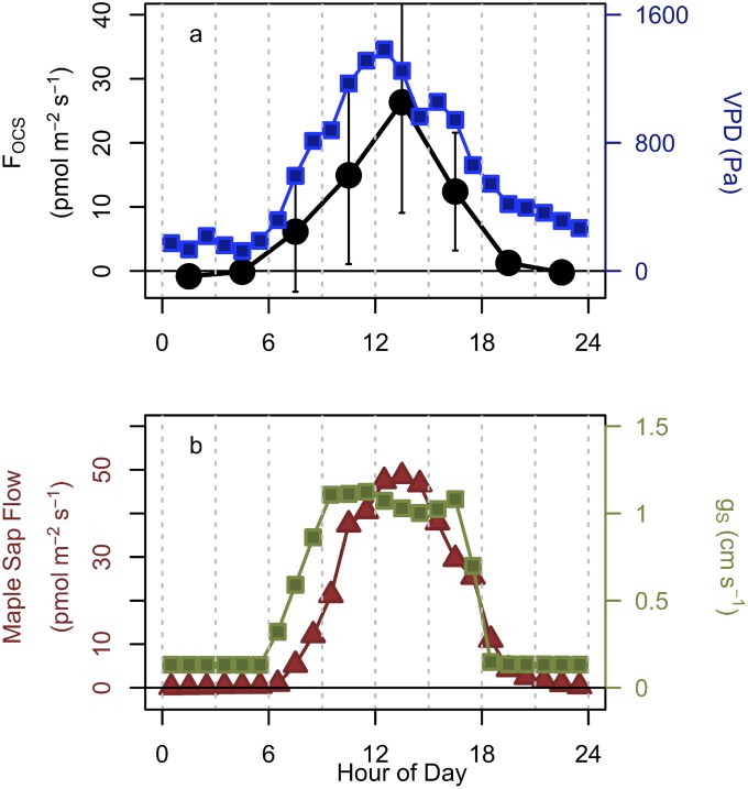
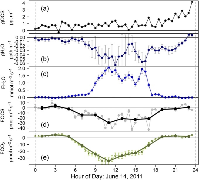
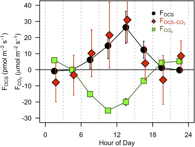
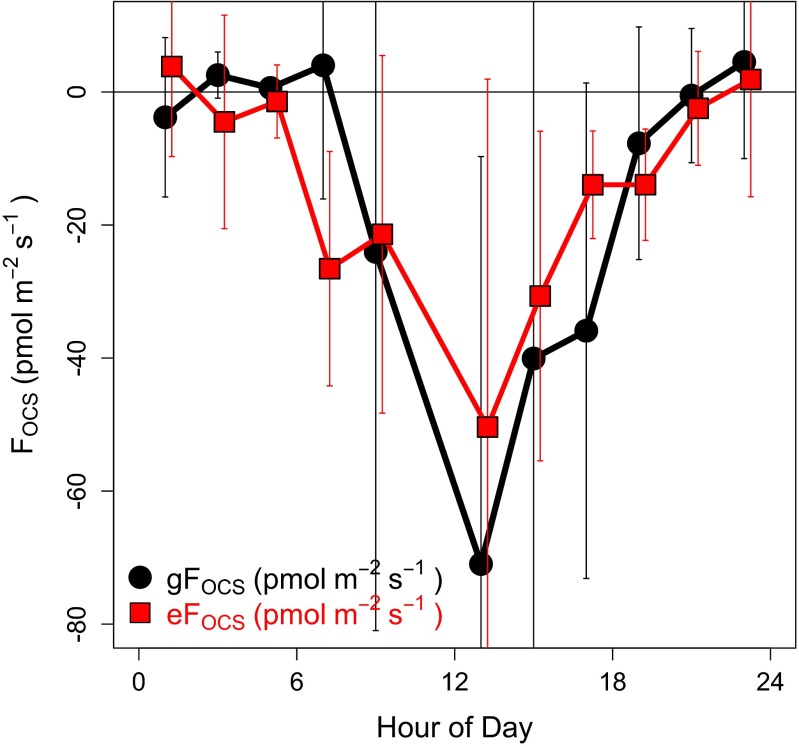
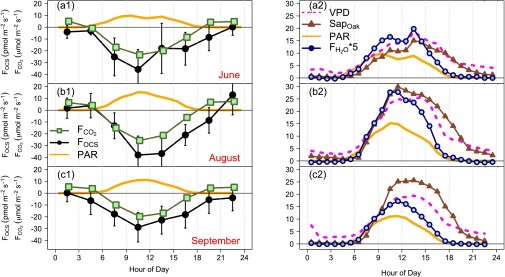
Carbonyl sulfide (OCS), the most abundant sulfur gas in the atmosphere, has a summer minimum associated with uptake by vegetation and soils, closely correlated with CO2. We report the first direct measurements to our knowledge of the ecosystem flux of OCS throughout an annual cycle, at a mixed temperate forest. The forest took up OCS during most of the growing season with an overall uptake of 1.36 ± 0.01 mol OCS per ha (43.5 ± 0.5 g S per ha, 95% confidence intervals) for the year. Daytime fluxes accounted for 72% of total uptake. Both soils and incompletely closed stomata in the canopy contributed to nighttime fluxes. Unexpected net OCS emission occurred during the warmest weeks in summer. Many requirements necessary to use fluxes of OCS as a simple estimate of photosynthesis were not met because OCS fluxes did not have a constant relationship with photosynthesis throughout an entire day or over the entire year. However, OCS fluxes provide a direct measure of ecosystem-scale stomatal conductance and mesophyll function, without relying on measures of soil evaporation or leaf temperature, and reveal previously unseen heterogeneity of forest canopy processes. Observations of OCS flux provide powerful, independent means to test and refine land surface and carbon cycle models at the ecosystem scale.

Keywords: carbon cycle; carbonyl sulfide; stomatal conductance; sulfur cycle.

Fig. 1.

Monthly mean OCS (F_OCS, pmol⋅m⁻²⋅s⁻¹; black) and CO₂ (F_CO2, µmol⋅m⁻²⋅s⁻¹; green squares) fluxes for 2011. u* > 0.17 m⋅s⁻¹ for all data. (A) Total OCS and CO₂ flux by month. Air temperature (red triangles; °C) and surface soil temperature (orange diamonds; °C); CO₂ net flux includes changes in storage, but this is not required for OCS. (B) Nighttime OCS (black) and CO₂ (green) flux (PAR < 40 µE⋅m⁻²⋅s⁻¹). (C) Daytime OCS and CO₂ fluxes with PAR > 600 µE⋅m⁻²⋅s⁻¹. Error bars indicate the 95% confidence intervals for all data within the month.

Fig. S1.

Comparison of OCS (pptv; pmol⋅mol⁻¹) measured by the TILDAS [30-min average (black) with 1σ SDs shown in gray], NOAA flask pair means [red points; 1σ SDs shown as red line error bars (barely visible)], and cosampled TILDAS OCS [3-h average at the time of the flask sample (gray circles)]. The flasks were sampled weekly followed by analysis by GC-MS in Boulder as part of the NOAA flask sample network (1).

Fig. S2.

The OCS (black circles; pmol⋅m⁻²⋅s⁻¹) flux, CO₂ flux (green squares; μmol⋅m⁻²⋅s⁻¹), and the air temperature (blue diamonds; °C) for given surface soil temperatures in December 2011. The data are partitioned to have equal numbers of data points for each temperature shown.

Fig. 2.

The relationship of OCS flux (F_OCS, pmol⋅m⁻²⋅s⁻¹; black circles), CO₂ flux (F_CO2, µmol⋅m⁻²⋅s⁻¹; green squares), and photosynthesis (calculated as GEP, µmol⋅m⁻²⋅s⁻¹; red triangles) with (A) air temperature and (B) PAR. Values of F_OCS and F_CO2 include nighttime values. (C) The ƒ_OCS/ƒ_GEP ratio with air temperature, for PAR > 300 µE⋅m⁻²⋅s⁻¹. (D) The ƒ_OCS/ƒ_GEP ratio with PAR, for PAR > 300 µE⋅m⁻²⋅s⁻¹. Black dashed lines show 95% CI. July data are excluded. Only data with u* > 0.17 m⋅s⁻¹ are used.

Fig. 3.

Monthly mean observed OCS (F_OCS Obs, pmol⋅m⁻²⋅s⁻¹; black) and Simple Biosphere (SiB3) model simulated OCS (F_OCS SiB, pmol⋅m⁻²⋅s⁻¹; red) fluxes for (A) daytime (PAR > 600 µE⋅m⁻²⋅s⁻¹) and (B) nighttime. (C) Mean diel cycle of observed (black) and simulated (red) OCS fluxes and stomatal conductance of OCS, g_S (cm⋅s⁻¹; green) for August–September 2011.

Fig. 4.

GEP calculated directly from OCS fluxes (GEP_OCS; yellow) with LRU values of 1 (brown long-dashed line), 1.5 (black points), and 2 (orange dashed line) and indirectly extrapolated from nighttime temperature-dependent respiration (GEP_CO2; green diamonds) for September 2011.

Fig. S3.

Diel cycles of (A) F_OCS (black circles; pmol⋅m⁻²⋅s⁻¹) and VPD (blue squares; Pa) and (B) bulk sap flow rate for maple trees (brown triangles; gH₂O⋅m⁻²⋅s⁻¹) and stomatal conductance (g_S; green squares; cm⋅s⁻¹) for the anomalous OCS emission period on July 19–31, 2011.

Fig. S4.

Components of gradient flux calculated OCS flux for June 14, 2011. (A) gOCS: OCS gradient (black; pptv⋅m⁻¹), confidence intervals of the OCS gradient (gray bars, which are barely visible). (B) gH₂O: H₂O gradient (dark blue; pptv⋅m⁻¹), confidence intervals of H₂O gradient (gray bars). (C) FH₂O: H₂O flux (blue; mmol⋅m⁻²⋅s⁻¹), 15% error on eddy covariance measurements (gray bars). (D) gFOCS: OCS gradient flux (pmol⋅m⁻²⋅s⁻¹), 2-h average (black), and 30-min gFOCS (gray points with SE as gray bars). (E) FCO₂: CO₂ flux (as NEE including storage contribution) (μmol⋅m⁻²⋅s⁻¹), 30-min FCO₂ (small light green points), 15% error on eddy covariance measurements (green bars), 2-h mean (dark green points).

Fig. S5.

Composite diel cycle of the gradient flux OCS derived from gradients of water vapor (F_OCS.H2O; black points) and carbon dioxide (F_OCS.CO2; red squares) for coincident data in 3 hourly time bins for July 19–31, 2011. The error bars indicate the 95% confidence intervals of the data within the composite 3-h period.

Fig. S6.

Composite diel cycle of the gradient flux OCS (gF_OCS; black points) and eddy covariance OCS flux (eF_OCS; red squares) for coincident data in 2 hourly time bins for August 6–12, 2011. The error bars indicate the 95% confidence intervals of the data within the composite 2-h period.

Fig. S7.

Diurnal composite of OCS (black) and CO₂ (green) fluxes (Eastern Standard Time) for the summer months of 2011: (A1) June, (B1) August, and (C1) September, with times of low turbulence (u* < 0.17 m⋅s⁻¹) removed. The 95% confidence intervals for each species are shown as black error bars. The 95% confidence intervals for CO₂ are barely visible. Both columns show PAR (solid orange line; 10⁻⁸ E⋅m⁻²⋅s⁻¹) on two different scales. A2, B2, and C2 show the sap flow rates for oak (brown triangles; gH₂O⋅m⁻²⋅s⁻¹), the vapor pressure deficit (magenta dashed line; Pa), and the water vapor flux [blue/navy circles; 5 mmol⋅m⁻²⋅s⁻¹ (multiplied by 5 for graphing)] for June, August, and September.

References

1. Montzka SA, et al. On the global distribution, seasonality, and budget of atmospheric carbonyl sulfide (COS) and some similarities to CO2. J Geophys Res. 2007;112(D9):D09302.
1. Barkley MP, Palmer PI, Boone CD, Bernath PF, Suntharalingam P. Global distributions of carbonyl sulfide in the upper troposphere and stratosphere. Geophys Res Lett. 2008;35(14):L14810.
1. Brühl C, Lelieveld J, Crutzen PJ, Tost H. The role of carbonyl sulphide as a source of stratospheric sulphate aerosol and its impact on climate. Atmos Chem Phys. 2012;12(3):1239–1253.
1. Berry J, et al. A coupled model of the global cycles of carbonyl sulfide and CO2: A possible new window on the carbon cycle. J Geophys Res Biogeosci. 2013;118(2):842–852.
1. Li X, Liu J, Yang J. Variation of H2S and COS emission fluxes from Calamagrostis angustifolia Wetlands in Sanjiang Plain, Northeast China. Atmos Environ. 2006;40(33):6303–6312. - PubMed
Publication types
LinkOut - more resources