A Bio-inspired Collision Avoidance Model Based on Spatial Information Derived from Motion Detectors Leads to Common Routes

Abstract

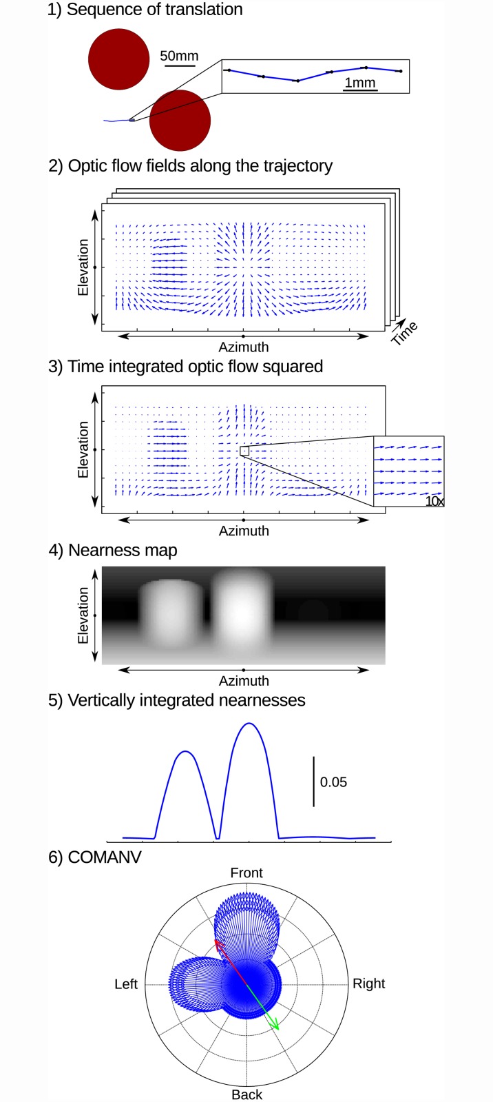
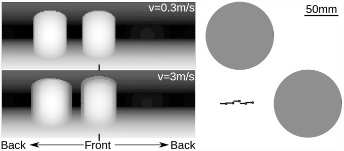
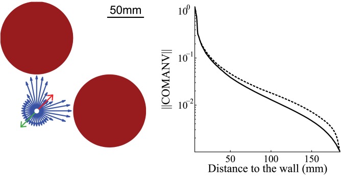
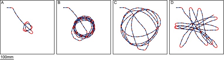
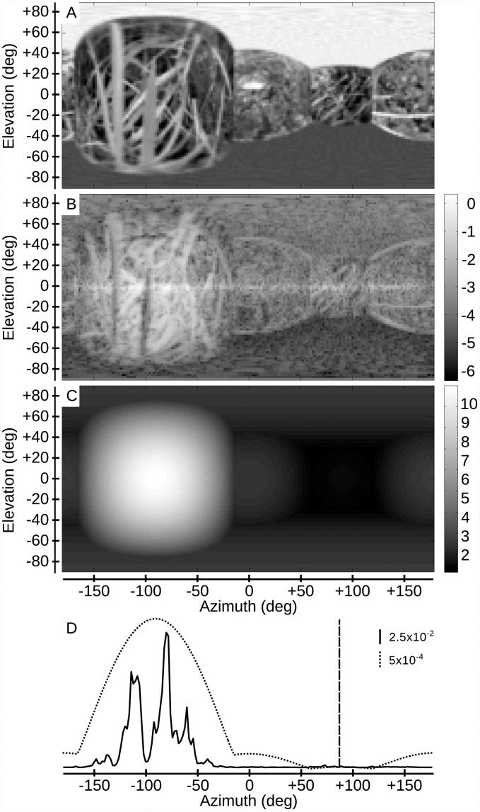
Avoiding collisions is one of the most basic needs of any mobile agent, both biological and technical, when searching around or aiming toward a goal. We propose a model of collision avoidance inspired by behavioral experiments on insects and by properties of optic flow on a spherical eye experienced during translation, and test the interaction of this model with goal-driven behavior. Insects, such as flies and bees, actively separate the rotational and translational optic flow components via behavior, i.e. by employing a saccadic strategy of flight and gaze control. Optic flow experienced during translation, i.e. during intersaccadic phases, contains information on the depth-structure of the environment, but this information is entangled with that on self-motion. Here, we propose a simple model to extract the depth structure from translational optic flow by using local properties of a spherical eye. On this basis, a motion direction of the agent is computed that ensures collision avoidance. Flying insects are thought to measure optic flow by correlation-type elementary motion detectors. Their responses depend, in addition to velocity, on the texture and contrast of objects and, thus, do not measure the velocity of objects veridically. Therefore, we initially used geometrically determined optic flow as input to a collision avoidance algorithm to show that depth information inferred from optic flow is sufficient to account for collision avoidance under closed-loop conditions. Then, the collision avoidance algorithm was tested with bio-inspired correlation-type elementary motion detectors in its input. Even then, the algorithm led successfully to collision avoidance and, in addition, replicated the characteristics of collision avoidance behavior of insects. Finally, the collision avoidance algorithm was combined with a goal direction and tested in cluttered environments. The simulated agent then showed goal-directed behavior reminiscent of components of the navigation behavior of insects.

Fig 1. Sketch of the algorithm from motion to CAD.

1) The motion of the agent consists of a series of translations in the null elevation plane. 2) Optic-flow fields along the trajectory contain FOEs and FOCs. 3) The time-integrated optic flow squared does not contain FOC and FOE. Inset is a 10× zoom at the mean motion direction of the agent. 4) Nearness map computed from time-integrated optic flow squared. 5) Nearness map averaged along the elevation. 6) Computation of the COMANV. Blue: representation of the vertically integrated nearness map in polar coordinates. Red: vectorial sum of the vertically integrated nearness vectors (COMANV). Green: vector directed opposite to the COMANV.

Fig 2. Blurred relative nearness of two cylindrical obstacles at high speed of the agent.

Left panels: Nearness maps computed from optic flow experienced during translation at a speed of 0.3ms⁻¹ and 3ms⁻¹. Right panel: Trajectory at the speed of 3ms⁻¹ towards one obstacle. Black circle and black line represent the head and the body of the agent, respectively. Gray circles represent the objects seen from above.

Fig 3. Direction and norm of COMANV.

Left panel: Direction of the COMANV. Blue, red and green vectors are nearness vector, +COMANV, and -COMANV, respectively. Red disks represent the objects. (The norms of the vectors have been scaled.) Right panel: Norm of COMANV as a function of the distance to the box wall. Box height: 390mm (solid line) and 3900mm (dashed line).

Fig 4. Closed-loop simulations of trajectories of the agent equipped with the collision avoidance algorithm in a cubic box.

Blue and red lines are intersaccades and saccades, respectively. A) The saccade amplitudes were computed such that the agent moves in the CAD after the saccade. B, C and D) The saccade amplitudes were computed such that the agent moves in a direction corresponding to only a fraction of the CAD after the saccade. The fraction of the CAD was computed with a sigmoid function, parameterized by a gain and a threshold, of the CAN. B) Gain = 2, Threshold = 1.6. C) Gain = 2, Threshold = 3.2 D) Gain = 10⁶, Threshold = 3.2.

Fig 5. EMD responses and nearness map.

A) Panoramic view of the environment, consisting of a cubic box covered with a natural grass texture, from the location where the nearness map was computed (front is azimuth 0°). B) log-scaled nearness map computed on the basis of EMD responses. C) Nearness map at the same location computed from the geometrical optic flow. D) Vertically integrated nearness map extracted respectively from EMD responses (solid line) and geometrical optic flow (dotted line). The vertical dashed line shows the CAD computed from the vertically integrated nearness map based on EMD responses. The direction matches the one computed with geometrical optic flow.

Fig 6. COMANV versus wall distance in a cubic box.

The box (height: 390mm) was covered with random checkerboard patterns of either 1mm (blue) or 4mm (green). Red: the box had a height of 3900mm and was covered with a 1mm random checkerboard pattern. Left panel shows the norm of the COMANV computed on the basis of EMD responses. Right panel shows the angle between the COMANV computed from EMD responses and the control based on geometrical optic flow. Thick lines and shaded area represent the mean and the standard deviation, respectively, computed at a given distance from the wall.

Fig 7. Trajectories of the agent with a collision avoidance system based on EMDs in a box (40 × 40 × 40cm) covered with different patterns (seen from above).

Trajectories with four different starting positions are shown (see S12 Fig for different starting position). The simulation time was 10sec or until the agent crashed. Walls of the box are covered with a natural pattern (A), a 1mm random checkerboard (B), a 4mm random checkerboard (C), an 8mm random checkerboard (D), a 35mm random checkerboard (E), and a random pattern with 1/f statistic (F). The gain and the threshold of the weighting function was 2 and 4, respectively, for all cases.

Fig 8. Trajectories of the agent with a collision avoidance system based on EMDs in a box (40 × 40 × 40cm) containing up to four objects and covered with different patterns (seen from above).

The pattern on the objects and wall were 1mm and 4mm random checkerboards for the top and bottom panels, respectively. A, D) One object in the center of the box. B, E) Two objects on one diagonal. C, F) Four objects on the diagonals. The objects were vertical bars with a quadratic base with a side length of 3cm and a height of 40cm. The gain and the threshold of the weighting function was 2 and 4, respectively, for all cases.

Fig 9. Trajectories of the agent equipped with an EMD-based collision avoidance system in two different cluttered environments with objects and the walls covered by 1mm random checkerboard patterns (seen from above).

Fifty-one starting positions were tested, and simulations were run for 100sec or until the agent crashed. The trajectories are color-coded depending on their starting position. Objects are indicated by filled black squares. The gain and the threshold of the weighting function was 2 and 4, respectively, for all cases. (see also S1 Video).

Fig 10. Trajectories of the agent equipped with an EMD-based collision avoidance system, but also relying on the goal direction, in two different cluttered environments with objects and walls covered by 1mm (right column) or 4mm (left column) random checkerboard patterns.

The goal is indicated by the green dot. Two hundred one starting positions were tested and simulations were run either for 100sec (gray lines, i.e. dead-end), until the goal was reached (colored lines) or until a crash occurred (black lines). Note that the individual trajectories converge to only a small number of distinct routes. Apart from taking the goal direction into account, the simulations, parameters and environments are identical to those used for Fig 9. (see also S2 Video,S3 Video).

Fig 11. A selection of the routes shown in Fig 10) for the two environments.

Although the area of starting positions greatly overlap for a given environment, the trajectories converge on two different routes (compare A with B, and C with D). The simulations, parameters and environments are identical to those used for the right panel of Fig 9.

Fig 12. Dendrogramm of route similarity for the two different cluttered environments, top and bottom row, respectively.

The routes followed by the agent (see Fig 9) are characterized by a cell sequence. Here, each cell is a triangle formed by neighboring objects. The route similarity is defined by the number of cells not shared by routes. First and second columns, path-similarity for 1mm and 4mm random checkerboard patterns, respectively. Third column, path-similarity across patterns. Note that identical routes are found for different patterns: for example, route #3 and route #2 in the first environment (top row) are identical to those for the environment covered by 1 mm and 4 mm random checkerboards, respectively. The routes are shown in S12 Fig,S13 Fig,S14 Fig,S15 Fig.

References

1. Chiang AS, Lin CY, Chuang CC, Chang HM, Hsieh CH, Yeh CW, et al. Three-Dimensional Reconstruction of Brain-wide Wiring Networks in Drosophila at Single-Cell Resolution. Current Biology. 2011;21(1):1–11. 10.1016/j.cub.2010.11.056 - DOI - PubMed
1. Witthöft W. Absolute anzahl und verteilung der zellen im him der honigbiene. Zeitschrift für Morphologie der Tiere. 1967;61(1):160–184. 10.1007/BF00298776 - DOI
1. Warzecha AK, Egelhaaf M. Response latency of a motion-sensitive neuron in the fly visual system: dependence on stimulus parameters and physiological conditions. Vision research. 2000;40(21):2973–2983. 10.1016/S0042-6989(00)00147-4 - DOI - PubMed
1. Egelhaaf M, Boeddeker N, Kern R, Kurtz R, Lindemann JP. Spatial vision in insects is facilitated by shaping the dynamics of visual input through behavioral action. Frontiers in neural circuits. 2012;6 10.3389/fncir.2012.00108 - DOI - PMC - PubMed
1. Surmann H, Lingemann K, Nüchter A, Hertzberg J. A 3D laser range finder for autonomous mobile robots. In: Proceedings of the 32nd ISR (International Symposium on Robotics). vol. 19; 2001. p. 153–158.
Publication types
LinkOut - more resources