Convergence, Divergence, and Reconvergence in a Feedforward Network Improves Neural Speed and Accuracy

Abstract

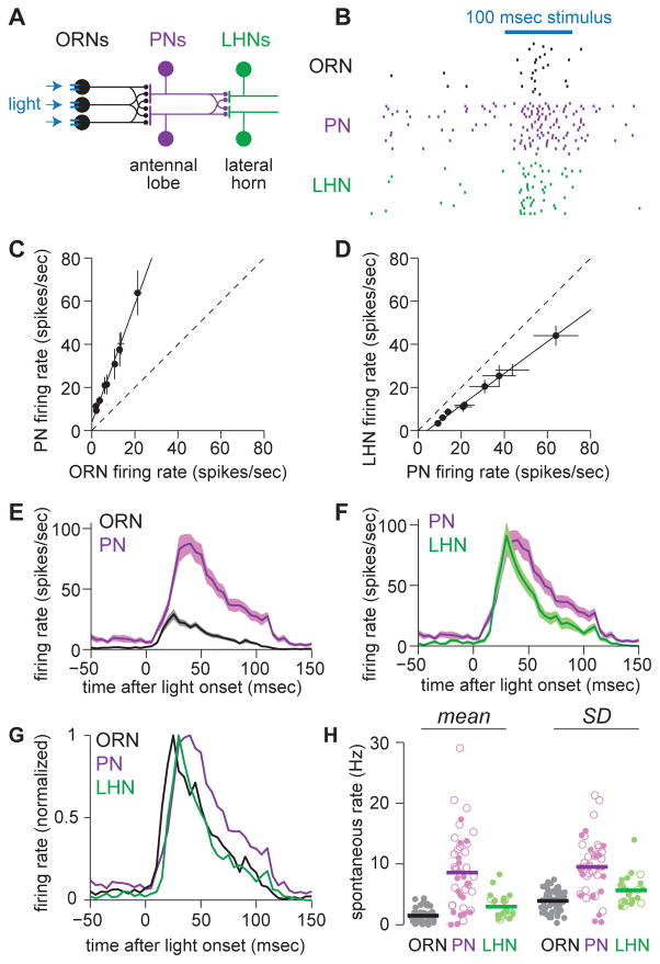
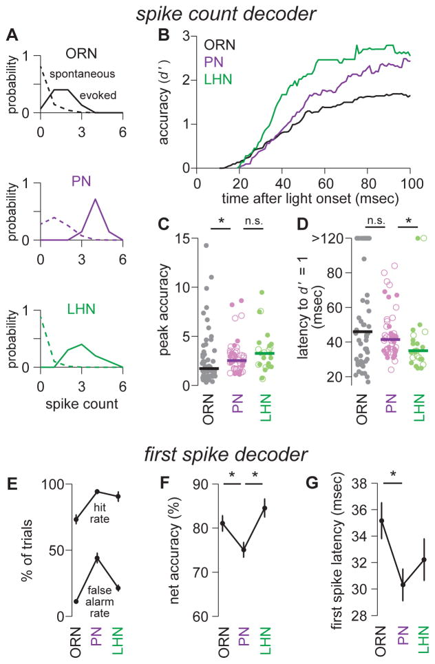
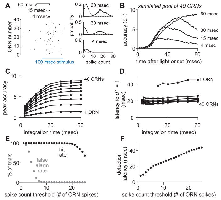
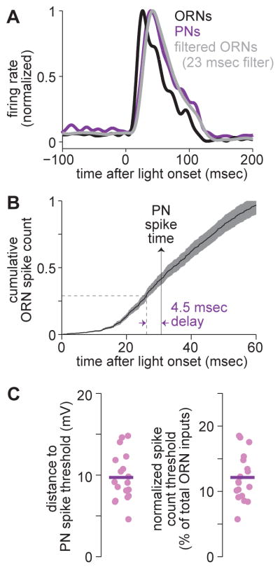
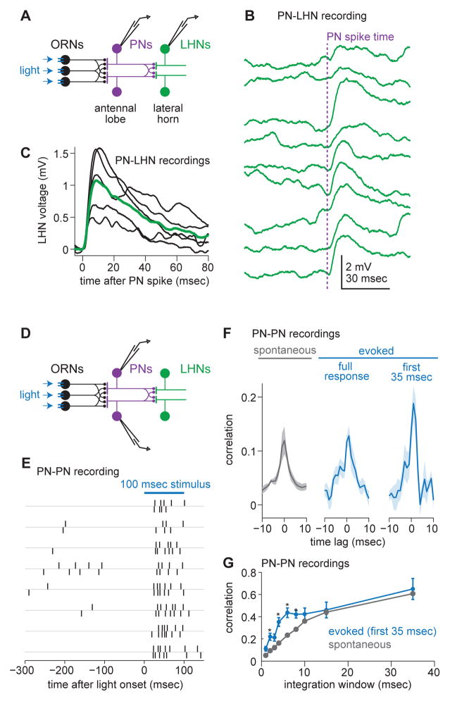
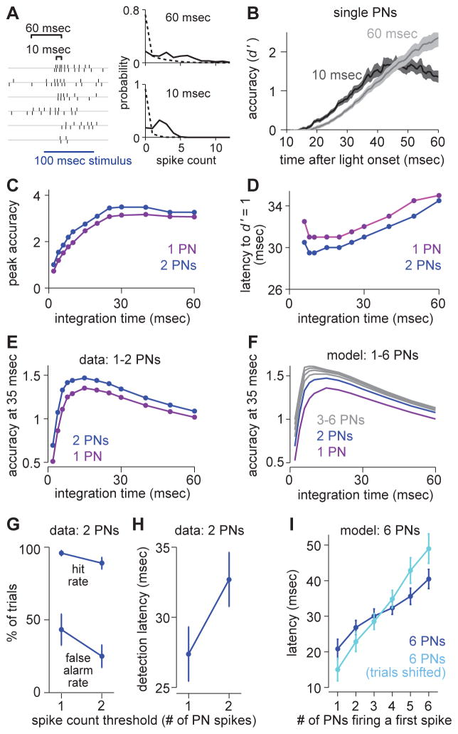
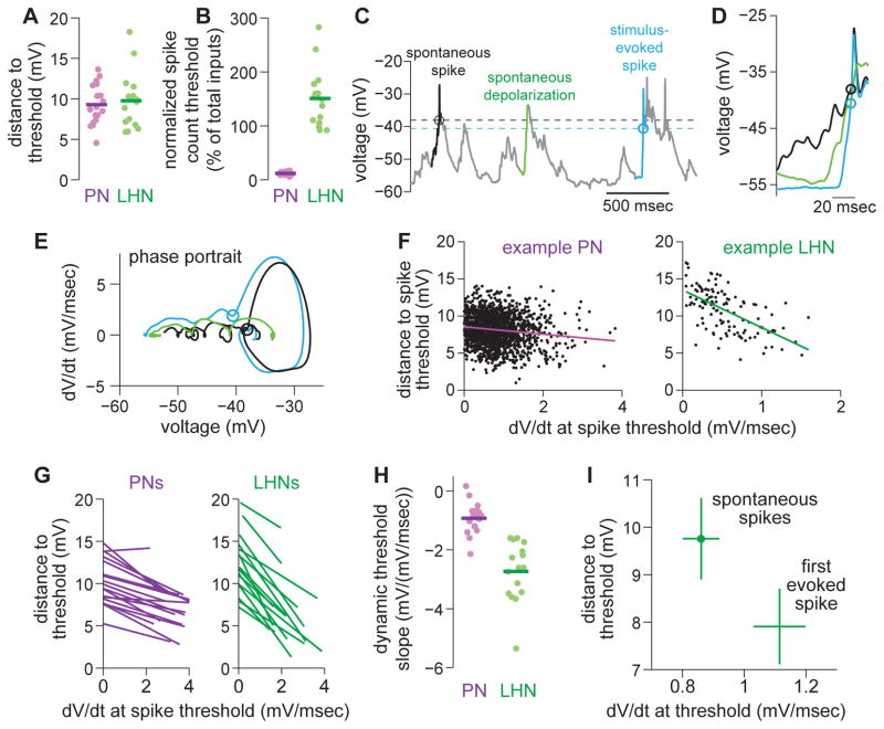
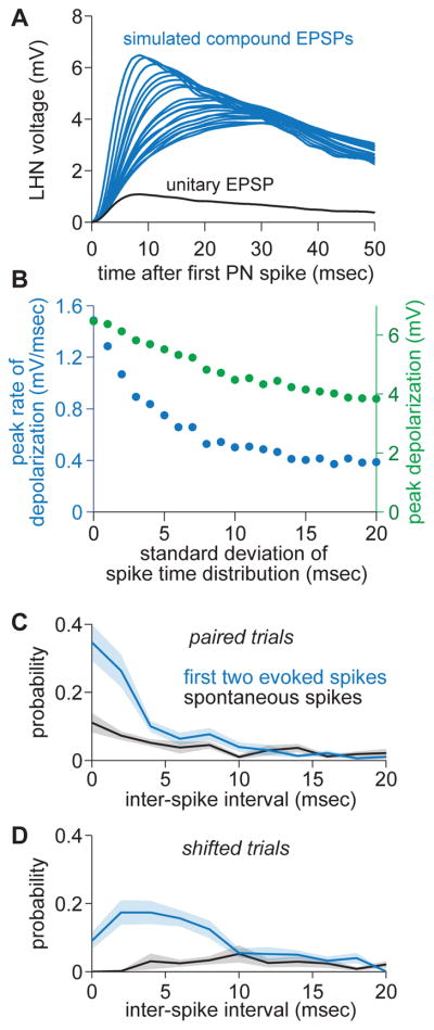
One of the proposed canonical circuit motifs employed by the brain is a feedforward network where parallel signals converge, diverge, and reconverge. Here we investigate a network with this architecture in the Drosophila olfactory system. We focus on a glomerulus whose receptor neurons converge in an all-to-all manner onto six projection neurons that then reconverge onto higher-order neurons. We find that both convergence and reconvergence improve the ability of a decoder to detect a stimulus based on a single neuron's spike train. The first transformation implements averaging, and it improves peak detection accuracy but not speed; the second transformation implements coincidence detection, and it improves speed but not peak accuracy. In each case, the integration time and threshold of the postsynaptic cell are matched to the statistics of convergent spike trains.

Figure 1. Sensory processing across three layers of olfactory circuitry

(A) Schematic of feedforward circuitry from a single olfactory glomerulus (DA1). About 40 ORNs in each antenna project to this glomerulus. Each ORN axon diverges to contact all the PNs in this glomerulus, and conversely each PN receives convergent input from all 40 ORNs. PN axons then reconverge onto LHNs. ORNs express channelrhodopsin-2, and we use light to inject a brief packet of spikes into the ORNs. (B) Rasters showing spikes in a DA1 ORN, a DA1 PN, and a postsynaptic LHN in response to repeated presentations of the primary stimulus used throughout this study (a 100 msec flash). (C) ORN and PN firing rates evoked by a range of optogenetic stimuli of different intensities. Each symbol represents a different stimulus. The open circle denotes the primary stimulus used throughout this study. Dashed line denotes unity slope. (D) As in (C), but for PN and LHN firing rates. PN-LHN gain is lower than ORN-PN gain (ANCOVA, p = 7.6 × 10⁻¹³). (E) Mean firing rate over time in ORNs and PNs (± s.e.m. across cells, n=58 ORNs and 44 PNs). (F) As in (E) but comparing PNs and LHNs (n=25 LHNs). (G) Mean firing rates from (E,F) normalized to their peak. (H) Spontaneous firing rates, mean (left) and standard deviation (right). Each symbol is a different recording (open circles are cell-attached recordings, filled circles are whole-cell current clamp recordings). Mean rates are higher in PNs than in ORNs (t-test, p = 2.4×10⁻¹³) or LHNs (t-test, p = 5.1×10⁻⁵). Standard deviations are also higher in PNs than in ORNs (t-test, 3.7×10⁻¹³) or LHNs (t-test, 3.0×10⁻⁴).

Figure 2. Multilayered circuitry improves accuracy and speed

(A) Spike count histograms for 80 msec time windows containing a stimulus (solid) or no stimulus (dashed). Data are accumulated across multiple trials for a typical ORN, PN, and LHN. The accuracy of stimulus detection is assessed using the metric d′. This value is the separation between the means of the two distributions (μ_evoked - μ_spontaneous) normalized by the root of the average variance of the two distributions (√(½ (σ²_evoked + σ²_spontaneous)). (B) Median accuracy (d′) over time for ORNs, PNs, and LHNs. An 80 msec window was slid forward in time, and resulting d′ values were plotted at the end point of each window. This and all subsequent panels in this figure are computed on the same data set (n=58 ORNs, 44 PNs, 25 LHNs). (C) Peak accuracy (d′) for individual ORNs, PNs, and LHNs. PNs are significantly different from ORNs (Wilcoxon rank-sum test, p = 0.013), but not significantly different from LHNs (Wilcoxon rank-sum test, p = 0.25). Solid bars denote medians. (PN detection accuracy is actually lower than our theoretical expectation, due to high spontaneous activity in PNs; see Figure S8.) (D) Latency to baseline detection accuracy (d′ =1) for individual ORNs, PNs, and LHNs. Latency is similar for ORNs and PNs (Wilcoxon rank-sum test, p = 0.33), but shorter for LHNs than for PNs (Wilcoxon rank-sum test, p = 0.015). Solid bars denote medians. (E) Mean hit rates and false alarm rates for a decoder operating with a threshold of a single spike (± s.e.m. across cells). The hit rate is the percentage of trials with at least one spike during the stimulus period. The false alarm rate is the percentage of trials with at least one spike during a period of equal length (100 msec) when no stimulus was presented. (F) Mean net accuracy for the decoder in E (± s.e.m. across cells). Net accuracy is worse for PNs than for ORNs (t-test, p = 0.018) or LHNs (t-test, p = 0.00077). Net accuracy is the average of the hit rate and the correct rejection rate. (G) Mean first spike latency (i.e., the detection latency for the decoder in E), ± s.e.m. across cells. Latency is shorter in PNs than in ORNs (t-test, p = 0.0092). Latency is not significantly different in PNs and LHNs (t-test, p = 0.32). Different methods of measuring first spike latency produced slightly different values but did not change the qualitative differences between cell types (see Supplemental Experimental Procedures, Data Analysis).

Figure 3. A decoder of ORN activity benefits from a long integration time and low threshold

(A) Comparing different integration windows by counting ORN population spikes in sliding windows of variable length (i.e., a variable integration time). At each time point, we construct spike count histograms and measure the separation between spontaneous and evoked activity (stimulus detection accuracy) using d′. (B) Mean accuracy (d′) over time for simulated populations of 40 ORNs. Increasing integration time increased peak accuracy. Populations were assembled by randomly selecting (without replacement) single trials from all of our ORN data (n = 58 ORN recordings, see Supplemental Experimental Procedures). (C) Peak accuracy for various integration times (mean over 2000 simulations of each ORN pool size). ORN pool sizes plotted are: 1, 5, 10, 15, 20, 25, 30, 35, and 40. (D) As in C, but for latency to baseline accuracy (d′ = 1). (E) Performance of a binary classifier (operating over 30 msec integration windows), for a range of spike count thresholds. (F) Detection latencies for the binary classifier in E, for a range of spike count thresholds.

Figure 4. PNs have a long integration time and a low spike count threshold

(A) Normalized firing rates for ORNs and PNs (reproduced from Figure 1G). Convolving the ORN response with a rectangular filter having a width of 23 msec yields a good fit to the PN response. (B) Mean cumulative ORN spike count (± s.e.m. across cells, n = 58). The vertical solid line with the arrow denotes mean time to first evoked PN spike (from Figure 2G). After accounting for the 4.5 msec transmission delay between ORN spikes and PN EPSP onset, the horizontal dashed line identifies that 0.28 spikes/ORN have occurred prior to the typical first PN spike. This is equivalent to about 11 spikes per 40 ORNs. (C) Distance to spike threshold. Left: distance in units of voltage, measured as the difference between the average threshold of spontaneous PN spikes and the average PN voltage overall (n = 18 PN recordings). Right: same data expressed as the percentage of all ORNs that must spike once to drive the PN to threshold (assuming a unitary EPSP amplitude of 2 mV and 40 ORNs, see Supplemental Experimental Procedures).

Figure 5. Individual lateral horn neurons pool input from sister PNs and stimulus onset increases short-timescale correlations among sisters

(A) Schematic of a paired PN-LHN recording. (B) Examples of unitary EPSPs recorded from a single LHN (green) in response to a single PN spike evoked by current injection (PN spike time indicated by vertical dashed line). Traces are ordered chronologically, top to bottom. (C) Mean EPSPs (black) for each paired recording. Overlaid is the grand average unitary EPSP over all 5 pairs. Before averaging, EPSPs are aligned to the time of the PN spike (specifically, the onset of the PN spike waveform; see Supplemental Experimental Procedures). On average, the latency between the PN spike and EPSP onset is 1.3 ± 0.2 msec (mean ± SEM across recordings; measured as the time that the trial-averaged EPSP in an LHN takes to reach 5% of its peak). (D) Schematic of a paired PN-PN recording. (E) Rasters from two simultaneously recorded DA1 PNs. (F) Cross-correlation functions (shift-subtracted) for spontaneous and stimulus-evoked activity (mean ± s.e.m. over pairs, n = 8 DA1 PN pairs). Stimulus evoked activity is shown for two time windows, one encompassing the full response (120 msec), and one that includes only the first 35 msec of the response. (G) Correlation coefficient (shift-subtracted) for PN pairs over various integration windows (mean ± s.e.m. over pairs). There is a significant effect integration window size on the correlation coefficient (ANOVA, p = 0.0061). For short integration windows, correlation coefficients are higher during evoked activity than during spontaneous activity (* denotes p < 0.02, paired t-test).

Figure 6. A decoder of PN population activity faces a speed-accuracy tradeoff

(A) Comparing different integration windows by counting spikes from pairs of PNs (or single PNs) in sliding windows of variable length (i.e., a variable integration time). At each time point, we construct spike count histograms and measure the separation between spontaneous and evoked activity (stimulus detection accuracy) using d′. (B) Accuracy (d′) over time based on spike trains from a single PN (mean ± s.e.m. over PNs). (C) Peak detection accuracy versus integration time, averaged over all PN pairs or the single PNs included in these pairs. Accuracy (single PNs) increases with integration time (ANOVA, p = 7.2 × 10⁻⁴). Accuracy is higher for PN pairs than for single PNs (ANOVA, p = 0.0142). This and all subsequent panels in this figure are computed on the same data set (n = 8 PN pairs). (D) Mean latency to baseline accuracy (d′ = 1) versus integration time. Latency increases with integration time (single PNs, ANOVA, p = 5.6 × 10⁻⁴). Latencies are shorter for PN pairs than for single PNs (ANOVA, p = 0.0090). Latency is not calculated for windows of 4 msec or shorter, because several (single) PNs never reach baseline accuracy. (E) Mean accuracy versus integration time, evaluated at 35 msec after stimulus onset. Accuracy is maximal for decoders that integrate over 10–20 msec. Accuracy is higher for PN pairs than for single PNs (ANOVA, p = 6.0 × 10⁻⁴). The improvement in accuracy with pairs is significantly greater for short timescales than for long timescales (ANOVA, interaction between population size and integration time: p = 0.0045). (F) Same as E but for modeled PN populations ranging in size from 1 PN to 6 PNs. Spike counts in PN populations were simulated based on distributions from paired PN data (Supplemental Experimental Procedures). (G) Hit rates and false alarm rates for a binary classifier (with a 10-ms integration window, mean ± s.e.m), for two different thresholds (one spike or two spikes, pooled over a pair of sister PNs). The higher threshold produces a higher net accuracy (paired t-test, p = 0.0189). (H) Detection latencies for the binary classifier in G, for the same two thresholds. The higher threshold imposes a speed cost of about 5 msec (paired t-test, p = 0.0073). (I) In a modeled population of 6 PNs, mean latency for a given number of these PNs to fire a first spike after stimulus onset. First PN spike distributions were simulated based on distributions from paired PN data (Supplemental Experimental Procedures). When trials were shifted to remove correlations, latencies became longer for higher thresholds.

Figure 7. LHNs operate with a high, but dynamic, spike count threshold

(A) Distance to spike threshold for PNs and LHNs. Each symbol is a different recording. This and subsequent group-data panels in this figure are computed on the same data set (n = 18 PNs and 16 LHNs). (B) Same but normalized by the estimated typical EPSP amplitude for each cell type (2 mV for PNs, 1.08mV for LHNs, see Figure 5C and Supplemental Experimental Procedures) and also normalized by the size of the presynaptic pool (here assumed to be 40 ORNs and 6 PNs). This value represents the percentage of the total presynaptic pool that must spike nearly-synchronously to drive the postsynaptic cell above threshold. (C) A typical whole-cell current clamp recording from an LHN highlighting two spikes (black and blue), and also a depolarization that does not evoke a spike (green). Circles and dashed lines denote spike thresholds. (D) Brief snippets of voltage surrounding the two spikes and the non-spiking depolarization (from C). (E) Phase portrait (dV/dt vs. V) for these three snippets. (F) Distance to spike threshold versus rate of depolarization for all spikes (spontaneous and stimulus-evoked) recorded from a typical PN and LHN. (G) Linear regression fits (like those in F) for all PNs and LHNs. Each line represents a different recording. (H) Slopes of linear regression fits from G for all PNs and LHNs. Distance to threshold depends on dV/dt more strongly in LHNs than in PNs (t-test, p = 1.9 × 10⁻⁷). (I) Distance to threshold versus dV/dt in LHNs. Spikes in two categories were analyzed—namely, spontaneous spikes and the first stimulus-evoked spike. Distance to threshold is significantly lower for the first stimulus-evoked spike (paired t-test, p = 6.2 × 10⁻⁴). dV/dt is also significantly higher for the first stimulus-evoked spike (paired t-test, p = 0.0024).

Figure 8. The dynamic threshold shortens the LHN integration window

(A) Simulated compound EPSPs in an LHN in response to 6 PN spikes with variable inter-spike intervals. A single unitary EPSP is shown in black for comparison. EPSP summation is assumed to be linear. (B) Comparison of the peak depolarization (green) and the peak rate of depolarization (blue) for the simulated compound EPSPs shown in A. The peak rate of depolarization falls off faster than does the peak depolarization. (C) In a pair of PNs, probability distributions of inter-spike intervals for the first two stimulus-evoked PN spikes, or the first two spontaneous PN spikes (measured from an arbitrarily chosen time point during spontaneous activity). The x-axis is truncated at 20 msec. (D) Same but for trial-shifted distributions, meaning correlations between sister PN pairs have been eliminated.

References

1. Alonso JM, Usrey WM, Reid RC. Precisely correlated firing in cells of the lateral geniculate nucleus. Nature. 1996;383:815–819. - PubMed
1. Averbeck BB, Latham PE, Pouget A. Neural correlations, population coding and computation. Nat Rev Neurosci. 2006;7:358–366. - PubMed
1. Azouz R, Gray CM. Dynamic spike threshold reveals a mechanism for synaptic coincidence detection in cortical neurons in vivo. Proc Natl Acad Sci U S A. 2000;97:8110–8115. - PMC - PubMed
1. Bair W, Zohary E, Newsome WT. Correlated firing in macaque visual area MT: time scales and relationship to behavior. J Neurosci. 2001;21:1676–1697. - PMC - PubMed
1. Bargmann CI. Comparative chemosensation from receptors to ecology. Nature. 2006;444:295–301. - PubMed
Publication types
MeSH terms
LinkOut - more resources