Estimation of passive and active properties in the human heart using 3D tagged MRI

Abstract

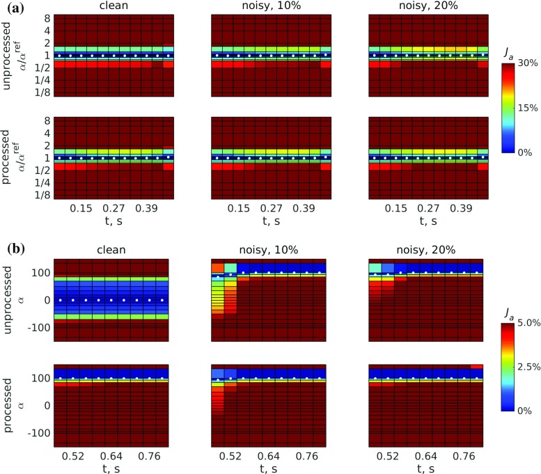
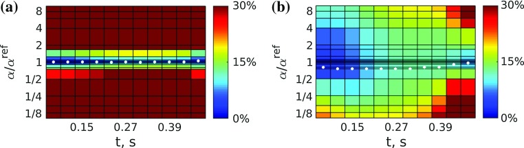
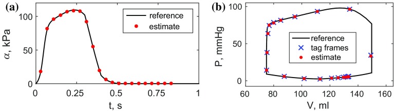
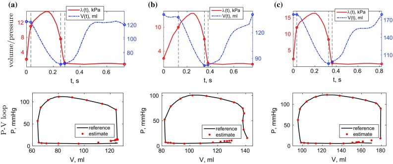
Advances in medical imaging and image processing are paving the way for personalised cardiac biomechanical modelling. Models provide the capacity to relate kinematics to dynamics and-through patient-specific modelling-derived material parameters to underlying cardiac muscle pathologies. However, for clinical utility to be achieved, model-based analyses mandate robust model selection and parameterisation. In this paper, we introduce a patient-specific biomechanical model for the left ventricle aiming to balance model fidelity with parameter identifiability. Using non-invasive data and common clinical surrogates, we illustrate unique identifiability of passive and active parameters over the full cardiac cycle. Identifiability and accuracy of the estimates in the presence of controlled noise are verified with a number of in silico datasets. Unique parametrisation is then obtained for three datasets acquired in vivo. The model predictions show good agreement with the data extracted from the images providing a pipeline for personalised biomechanical analysis.

Keywords: 3D tagged MRI; Cardiac mechanics; Parameter estimation; Patient-specific modelling.

Fig. 1

Idealised geometry in undeformed and deformed states through the cardiac cycle. a Reference geometry, b reference mesh, c end-diastolic mesh, d mid-systolic mesh, e end-systolic mesh

Fig. 2

Comparison of in silico datasets in mid-systole (long- and short-axis views). The surfaces show the domain deformed using clean displacement data, while the lines crossing the surfaces show the mesh deformed using the six different datasets produced for testing: clean unprocessed, unprocessed with noise at 10 and 20 % standard deviation, clean processed and processed noisy at 10 and 20 % standard deviation. Surface shading represents the distance between the clean displacements and the displacement for each of the cases. a Clean, b noisy, 10 % std, c noisy, 20 % std, d clean tags, e noisy tags, 10 % std, f noisy tags, 20 % std, g processed clean, h processed noisy, 10 % std, i processed noisy, 20 % std

Fig. 3

Reference data used in in silico tests: volume and active tension curves are constructed based on typical behaviour, and pressure curve is computed using the model. The crosses on the volume curve correspond to 3D tagged image frames. a Volume and pressure, b active tension, c P–V loop

Fig. 4

Variation of the objective function ${\mathcal{J}}_p$ over the space of the passive parameter ratio $\mathit{\gamma }({\mathit{\gamma }}^{\text{ref}}=0.1)$. The position of the minimum is indicated by a circle. Each data point corresponds to a single simulation run. a Unprocessed, b processed

Fig. 5

Variation of the objective function ${\mathcal{J}}_a$: a over the $\mathit{\alpha }/{\mathit{\alpha }}^{\text{ref}}$ space in systole, when ${\mathit{\alpha }}^{\text{ref}}>0$, and b over the $\mathit{\alpha }$ space in diastole, when ${\mathit{\alpha }}^{\text{ref}}=0$. White dots indicate positions of the minima for each step

Fig. 6

Comparison of the variation of a the objective function ${\mathcal{J}}_a$ combining relative displacement and pressure errors, and b the objective function consisting of relative displacement errors only for processed displacements with 20 % noise. White dots indicate positions of the minima for each step. Sharper variation around the minimum translates to better identifiability of the active parameter $\mathit{\alpha }$. a Displacement and pressure, b displacement only

Fig. 7

Comparison of the clean reference data and estimates for a the active tension scaling and b the P–V loop for the processed displacements with 20 % noise. a Active scaling, b P–V loop

Fig. 8

Reference volume data for the in vivo cases computed from the deformed meshes, and reference pressure data obtained by scaling the normalised curve (Russell et al. 2012) using mitral and aortic valve opening and closing times (vertical dashed lines). Dots on the P–V loop figures indicate the values produced by the model

Fig. 9

Variation of the objective function ${\mathcal{J}}_p$ over the passive parameter ratio space in the in vivo cases, with minima shown as circles

Fig. 10

Variation of the objective function ${\mathcal{J}}_a$ over the $\mathit{\alpha }$ space for each time step in the in vivo cases, with minima shown as white dots. Each vertical line corresponds to a single ${\mathcal{J}}_a$ over $\mathit{\alpha }$ plot for a given time t. For clear presentation of the minima in a combined plot over all time steps, the values of ${\mathcal{J}}_a$ were scaled to [0,1] for each t, and the shading corresponds to these scaled values. The range of the absolute values of ${\mathcal{J}}_a$ is given in Table 5. a V, b P1, c P2

Fig. 11

Mesh configurations through the cycle based on the model with estimated passive and active parameters (black) and motion tracking in the 3D tagged image set for case V. a End diastole, b mid-systole, c end systole, d mid-diastole, e late diastole

Fig. 12

Reference meshes obtained by deflation of the end-diastolic mesh using the passive parameter ratios c $\mathit{\gamma }=0.05$ and d $\mathit{\gamma }=1$ compared to a the end-diastolic mesh and b the end-systolic mesh used as the reference state in the main body of the paper

Fig. 13

Variation of the modified objective function ${\widehat{\mathcal{J}}}_p$ over the space of the passive parameter ratio based on estimated reference states for each ratio. The minimum is shown as a circle. The figures show the functional including a all diastolic frames starting at end systole, b all diastolic frames starting 3 frames past end systole, c only the end-diastolic frame

Fig. 14

Effect of changing fibre distributions on passive estimation for in vivo case V

Fig. 15

Estimated active tension using fibre-only activation, and fibre and transverse activation for case V

References

-
- Asner L, Hadjicharalambous M, Lee J, Nordsletten D (2015) STACOM Challenge: simulating left ventricular mechanics in the canine heart. In: Statistical atlases and computational models of the heart-imaging and modelling challenges, vol 8896. Springer, pp 123–134
- Babuska I. The finite element method with Lagrangian multipliers. Numer Math. 1973;20(3):179–192. doi: 10.1007/BF01436561. - DOI
- Bonet J, Wood R. Nonlinear continuum mechanics for finite element analysis. Cambridge: Cambridge University Press; 2008.
- Brenner SC, Scott R. The mathematical theory of finite element methods. Berlin: Springer; 2008.
Publication types
MeSH terms
Grants and funding
LinkOut - more resources
Full Text Sources
Other Literature Sources