Mirrored STDP Implements Autoencoder Learning in a Network of Spiking Neurons

Abstract

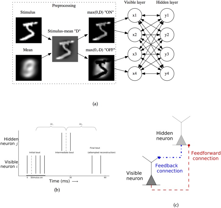
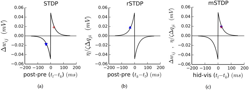
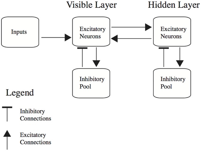
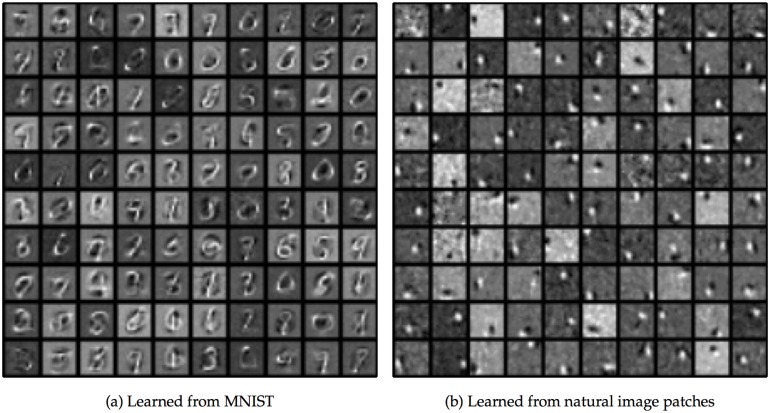
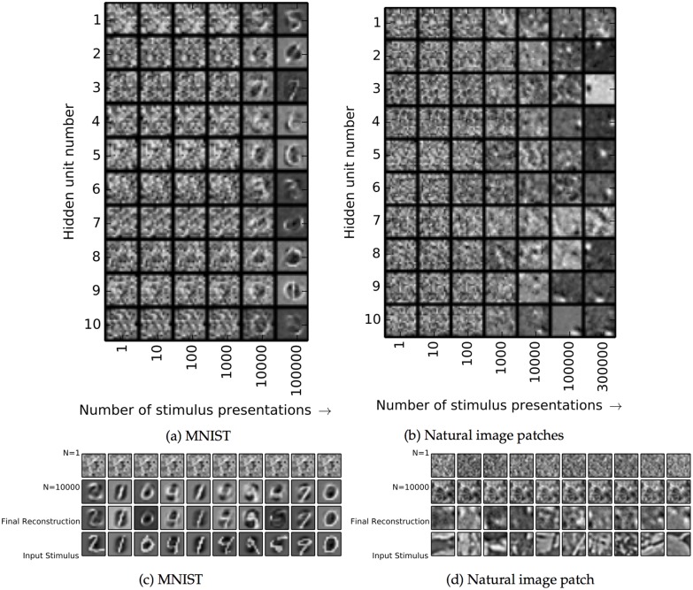
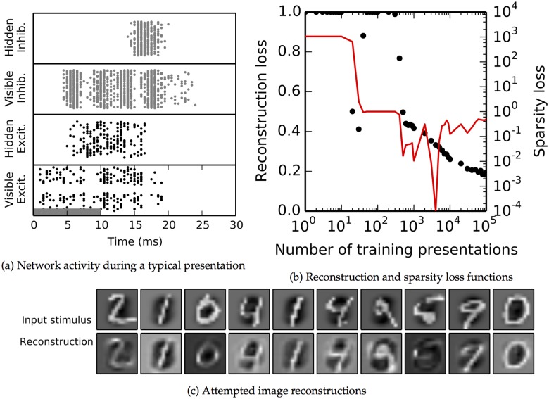
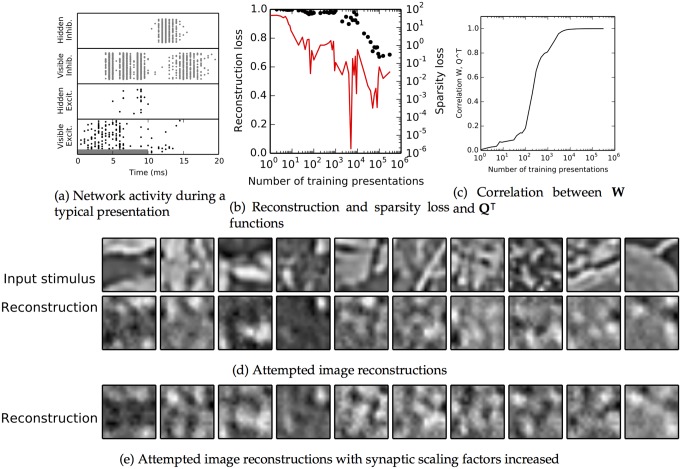
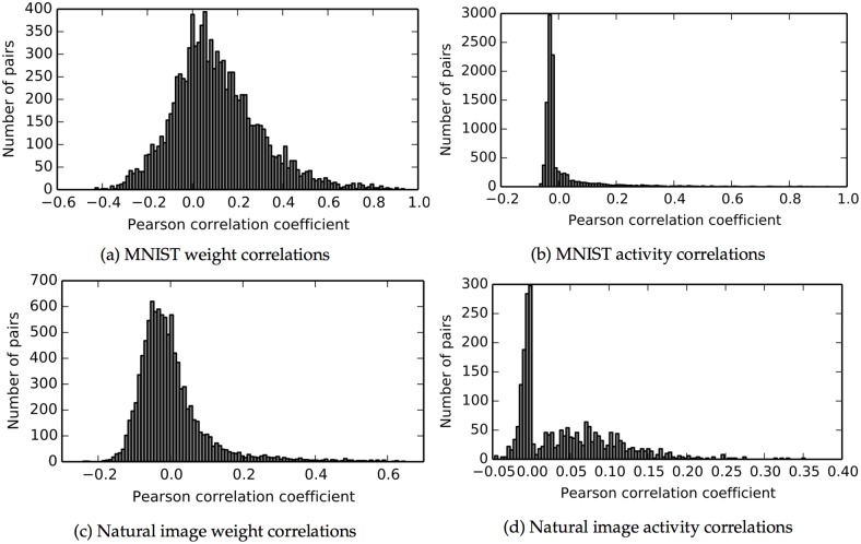
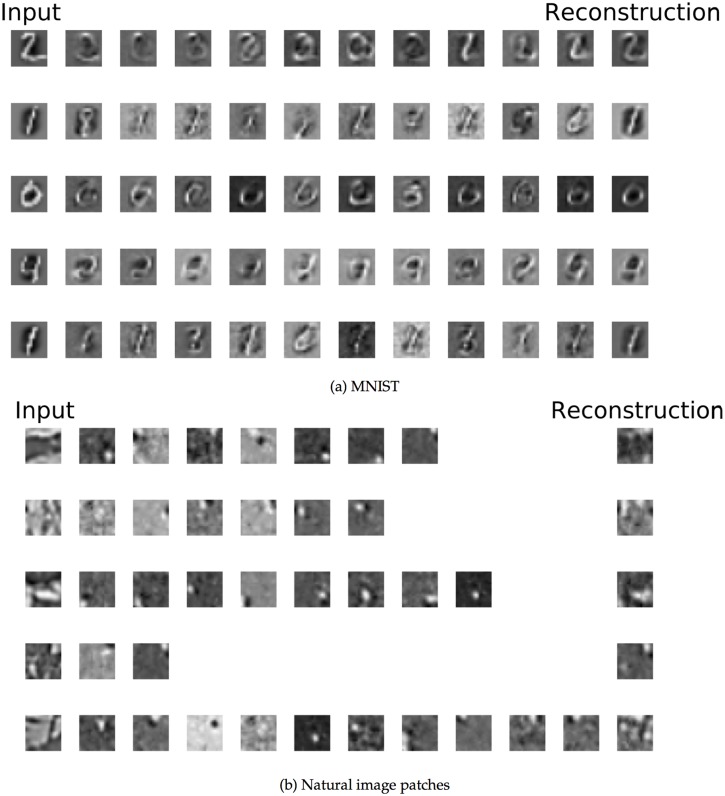
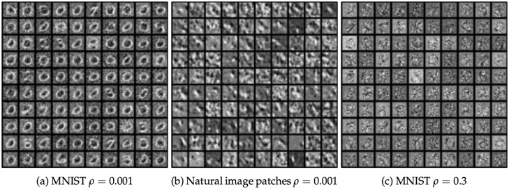
The autoencoder algorithm is a simple but powerful unsupervised method for training neural networks. Autoencoder networks can learn sparse distributed codes similar to those seen in cortical sensory areas such as visual area V1, but they can also be stacked to learn increasingly abstract representations. Several computational neuroscience models of sensory areas, including Olshausen & Field's Sparse Coding algorithm, can be seen as autoencoder variants, and autoencoders have seen extensive use in the machine learning community. Despite their power and versatility, autoencoders have been difficult to implement in a biologically realistic fashion. The challenges include their need to calculate differences between two neuronal activities and their requirement for learning rules which lead to identical changes at feedforward and feedback connections. Here, we study a biologically realistic network of integrate-and-fire neurons with anatomical connectivity and synaptic plasticity that closely matches that observed in cortical sensory areas. Our choice of synaptic plasticity rules is inspired by recent experimental and theoretical results suggesting that learning at feedback connections may have a different form from learning at feedforward connections, and our results depend critically on this novel choice of plasticity rules. Specifically, we propose that plasticity rules at feedforward versus feedback connections are temporally opposed versions of spike-timing dependent plasticity (STDP), leading to a symmetric combined rule we call Mirrored STDP (mSTDP). We show that with mSTDP, our network follows a learning rule that approximately minimizes an autoencoder loss function. When trained with whitened natural image patches, the learned synaptic weights resemble the receptive fields seen in V1. Our results use realistic synaptic plasticity rules to show that the powerful autoencoder learning algorithm could be within the reach of real biological networks.

Fig 1. Architecture of the model network and stimulus preprocessing.

Architecture of the model network and network activity. a: Architecture of the model network and stimulus preprocessing. The final preprocessing step of separating the stimulus into two non-negative “ON” and “OFF” populations allows the visible layer activities to remain positive. b: Example activity of two neurons in the spiking network. In response to external stimulus onset (gray bar), the visible neuron i fires several spikes in the “initial bout” of activity. After a delay, feedforward excitation causes the hidden neuron j to fires spikes in the “intermediate bout”. After another delay, feedback causes the visible neuron to spike in the “final bout”, the network’s attempted reconstruction. The average time between spikes in the initial and intermediate bouts and intermediate and final bouts are given by Δt ₁ and Δt ₂, respectively. Every pair of visible and hidden spikes contributes to plasticity, dependent on their relative times. Learning from two example dotted spikes is described in Fig 2. c: Biological feedforward and feedback connections are physically distinct. For the feedforward connection, the visible neuron is pre-synaptic, the hidden neuron is post-synaptic, and the synapse lies close to the hidden neuron’s cell body. For the feedback connection, the hidden neuron is pre-synaptic, the visible neuron post-synaptic, and the synapse is far out on the visible neuron’s dendritic tree.

Fig 2. Plasticity rules.

Each plot shows plasticity from spikes k and l from a visible and hidden neuron, respectively, which occur at times t _k and t _l. Red cross and blue triangle show learning from the two example dashed spikes in Fig 1b for feedforward and feedback connections, respectively. Note different x-axes on each plot. a: Standard STDP rule. Used for feedforward connections in the model, for which spike l is post-synaptic. x-axis shows time difference between post- and pre-synaptic spikes. The example spikes would strengthen the feedforward connection (red cross) but weaken the feedback connection, if feedback followed this rule (blue triangle). b: aSTDP rule, in which the time dependence is reversed. Used for feedback connections, for which spike k is post-synaptic. Learning rate is scaled by a constant ζ/η relative to STDP. c: Combined mSTDP rule. x-axis shows time difference between hidden and visible spikes, leading to identical profiles for STDP and aSTDP. Feedforward and feedback learning is symmetric (red cross and blue triangle).

Fig 3. Model architecture for the integrate-and-fire simulations, including pools of inhibitory neurons in each layer.

Fig 4. Feedforward weights after training for the MNIST and natural image patch datasets.

a: Weights learned from the MNIST dataset. Each square in the grid represents the incoming weights to a single hidden unit; weights to the first 100 hidden units are shown. Weights from visible neurons which receive OFF inputs are subtracted from the weights from visible neurons which receive ON inputs. Then, weights to each neuron are normalized by dividing by the largest absolute value. b: Same as (a), but for the natural image patch dataset.

Fig 5. Evolution of weights and reconstructions in the spiking model.

a–b: Evolution of weights in the spiking model. Weights as learned after different numbers of stimulus presentations are shown for 10 example hidden units. c–d: Attempted reconstructions at different points in training for the two spiking model experiments, for the stimuli shown in the bottom rows. Early in training, the same few hidden units whose incoming weights happened to be strongest were often activated regardless of the stimulus, leading to similar reconstruction attempts for different stimuli (first rows). Over time, the attempted reconstructions came to resemble the input stimuli.

Fig 6. Behavior of the simulated spiking network for the MNIST dataset.

a: Behavior of the network during a typical image presentation; compare with Fig 1b. Time period of external stimulation shown by grey bar. Raster plot includes all neurons which fired at least one spike during the presentation. The spikes of the visible neurons are in the bottom row and those of the hidden neurons are directly above. The top two rows, in grey, show the spikes for the inhibitory pools at each layer. Although the each training presentation ran for 65ms, all spikes occurred before 30ms so the raster plot was ended there. b: Reconstruction loss function, black dots, (defined in text) decreases over time, as does sparsity loss function (red, note log scale on y axis). c: The trained networks’ attempted reconstruction of representative training images. Each image shows the ON cell values minus the OFF cells. The first row shows the inputs to the network. The second row shows the attempted reconstruction ${\mathbf{Q}}^{⊺}\overrightarrow{z}$.

Fig 7. Behavior of the simulated spiking network for the natural image patch dataset.

a–d: As Fig 6, with addition of c, which shows the Pearson correlation coefficient between the feedback weights Q and the feedforward weights W as they become symmetric over time. Because of the sparsity constraint on learning, the network cannot learn a perfect representation, so final autoencoder loss is still quite large (b), but the network nevertheless captures many salient features when attempting reconstruction (d). e: Reconstruction attempts for the same input stimuli as in (d), when the scaling factors Φ_j were uniformly multiplied by 1.5 after training.

Fig 8. Hidden unit correlations after training.

Neither the incoming weights nor the spiking activity is uncorrelated between hidden units. a: Correlations of the final trained synaptic weights between every pair of hidden units in the MNIST network. b: Correlations of the spike numbers from 1,000 stimulus presentations between every pair of hidden neurons for MNIST. c–d: Same, for the natural image network.

Fig 9. Highly activated weights for example image presentations in the two datasets.

a: Weights for the MNIST dataset. First column shows 5 example inputs. Next 10 columns show the receptive fields of the 10 hidden units most activated for that input. Opacity codes the relative strength of the hidden unit’s responses with respect to the most active hidden unit; weakly activated hidden units are drawn nearly transparent. Final column shows the network’s attempted construction as measured by the late-time spike count. b: Same as (a), but for the the natural image patch dataset.

Fig 10. Learned hidden unit weights for different target activation rates ρ.

a: Learned weights for the MNIST dataset with ρ = 0.001. b: Learned weights for the natural image patch dataset with ρ = 0.001. c: Learned weights for the MNIST dataset with ρ = 0.3.

References

1. Kohonen T. Self-organized formation of topologically correct feature maps. Biol Cybern. 1982;43(1):59–69. 10.1007/BF00337288 - DOI
1. Sirosh J, Miikkulainen R. Cooperative self-organization of afferent and lateral connections in cortical maps. Biol Cybern. 1994;71(1):65–78. 10.1007/BF00198912 - DOI
1. Choe Y, Miikkulainen R. Self-organization and segmentation in a laterally connected orientation map of spiking neurons. Neurocomputing. 1998. November;21(1–3):139–158. 10.1016/S0925-2312(98)00040-X - DOI
1. Delorme A, Perrinet L, Thorpe SJ. Networks of integrate-and-fire neurons using Rank Order Coding B: Spike timing dependent plasticity and emergence of orientation selectivity. Neurocomputing. 2001. June;38–40:539–545. 10.1016/S0925-2312(01)00403-9 - DOI
1. Masquelier T, Thorpe SJ. Unsupervised learning of visual features through spike timing dependent plasticity. PLOS Comput Biol. 2007. February;3(2):e31 10.1371/journal.pcbi.0030031 - DOI - PMC - PubMed