. 2015 Dec 4;10(12):e0144404.
doi: 10.1371/journal.pone.0144404. eCollection 2015.

Extending Ripley's K-Function to Quantify Aggregation in 2-D Grayscale Images

Affiliations

Extending Ripley's K-Function to Quantify Aggregation in 2-D Grayscale Images

Mohamed Amgad et al. PLoS One. .

Abstract

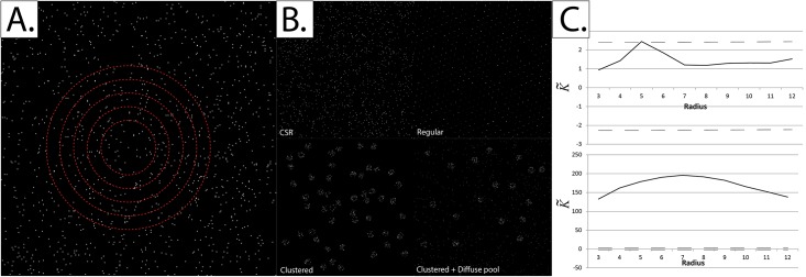
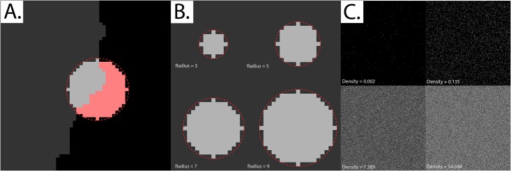
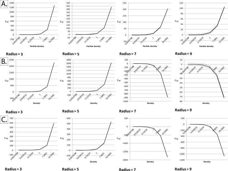
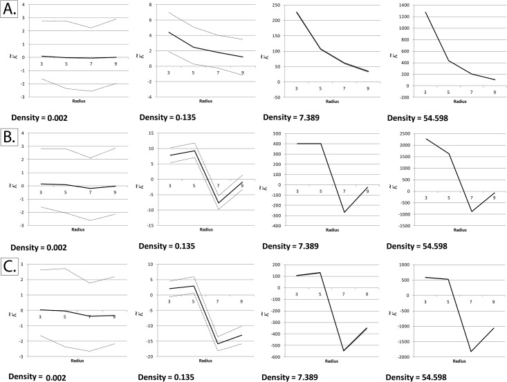
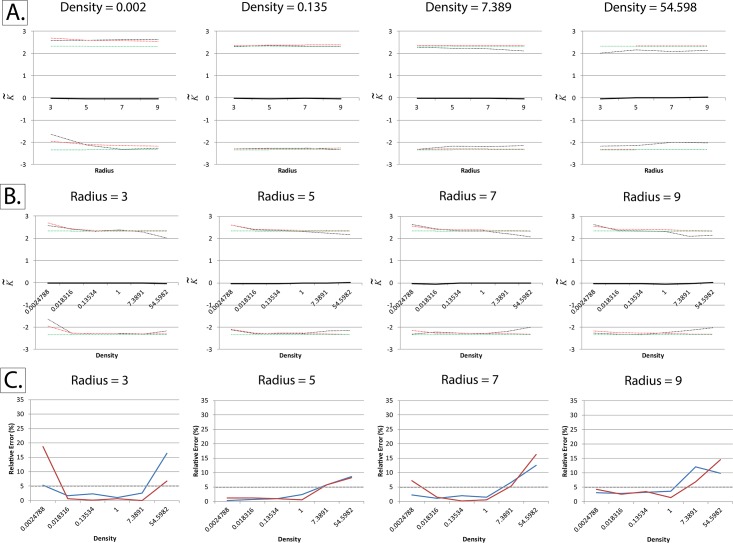
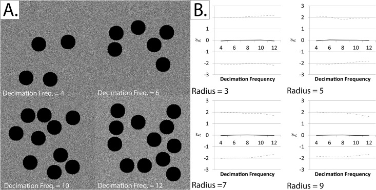
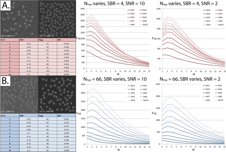
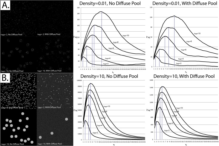
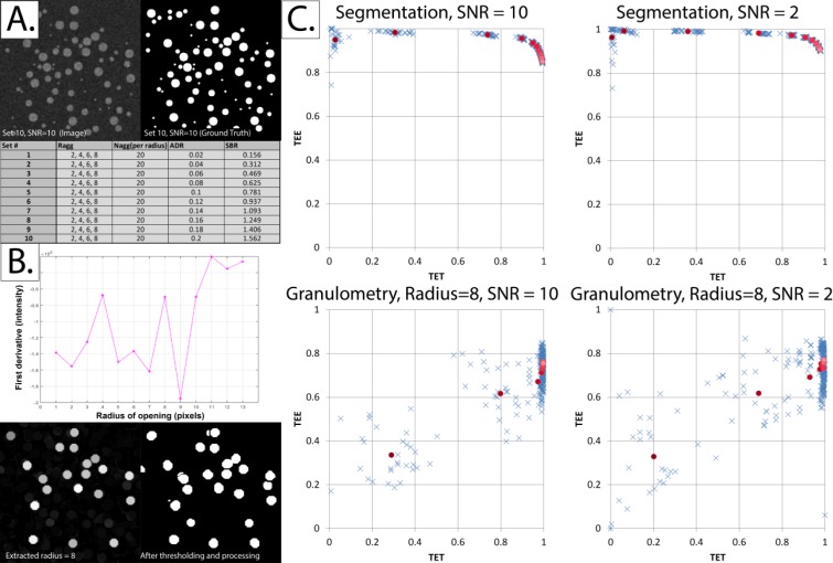
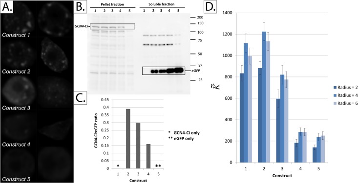
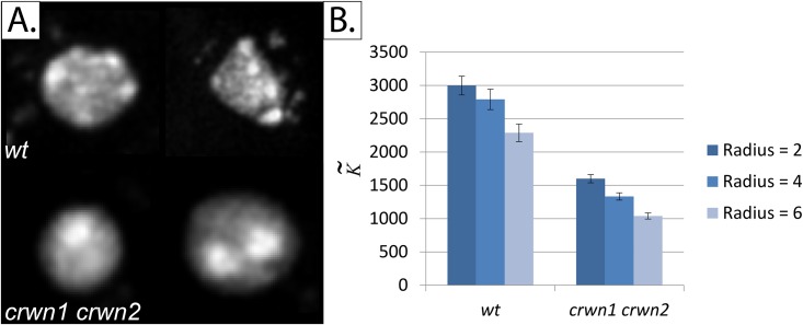
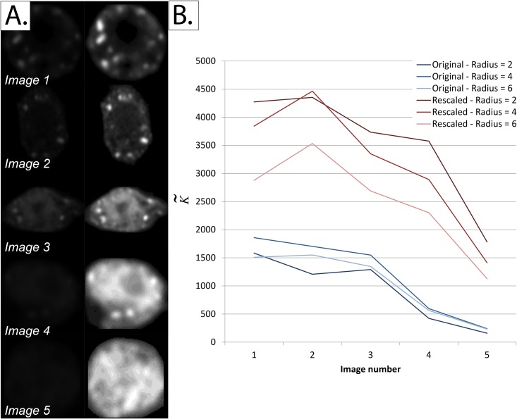
In this work, we describe the extension of Ripley's K-function to allow for overlapping events at very high event densities. We show that problematic edge effects introduce significant bias to the function at very high densities and small radii, and propose a simple correction method that successfully restores the function's centralization. Using simulations of homogeneous Poisson distributions of events, as well as simulations of event clustering under different conditions, we investigate various aspects of the function, including its shape-dependence and correspondence between true cluster radius and radius at which the K-function is maximized. Furthermore, we validate the utility of the function in quantifying clustering in 2-D grayscale images using three modalities: (i) Simulations of particle clustering; (ii) Experimental co-expression of soluble and diffuse protein at varying ratios; (iii) Quantifying chromatin clustering in the nuclei of wt and crwn1 crwn2 mutant Arabidopsis plant cells, using a previously-published image dataset. Overall, our work shows that Ripley's K-function is a valid abstract statistical measure whose utility extends beyond the quantification of clustering of non-overlapping events. Potential benefits of this work include the quantification of protein and chromatin aggregation in fluorescent microscopic images. Furthermore, this function has the potential to become one of various abstract texture descriptors that are utilized in computer-assisted diagnostics in anatomic pathology and diagnostic radiology.


Conflict of interest statement

Competing Interests: The authors have declared that no competing interests exist.

Figures

Fig 1
Fig 1. The concept behind Ripley’s K-function.
Panel A: Ripley’s K-function is defined as the average number of events within a predefined radius of any event, normalized for the event intensity (density) over the whole field of view. A set of radii is typically used to quantify the scale at which clustering (or dispersion) of events occurs (red circles). Panel B: Events within a given field of view could be distributed in many forms, including Complete Spatial Randomness (CSR), regularity and clustering (with or without a diffuse pool). Panel C: K˜ plots for two of the event distributions in Panel B: CSR (upper) and Clustering (lower). The dashed lines represent the upper and lower critical quantiles (Q01 and Q99).
Fig 2
Fig 2. Approaching problematic edge effects at non-binary fields of view and small radii.
Panel A: Three implementations of Besag’s edge correction term were tested. Note that the black region (black pixels) are considered to be outside the study region (i.e. the border between the grey and black area represents the edge of the study region), The implementations are as follows: i) Dividing the total number of pixels, located within a pre-defined radius from a given border pixel (light-gray area), by the total area of an ideal circle (area enclosed by the dotted red line). ii) Same as implementation i, but dividing by the total area of a non-ideal/pixelated circle (light-gray plus pink regions). iii) Same as implementation i, but applied for all pixels within the field of view. Hence, even for non-border pixels, the edge correction term would be obtained by dividing the area of the pixelated circle by the area of a perfect circle of the same radius. Panel B: The difference between an “ideal” circle and its pixelated counterpart at the four radii tested in this paper. Panel C: Complete Spatial Randomness (CSR) at a selected number of event densities (intensities). Each field of view measures 256 x 256 pixels. The image intensities were re-scaled for display purposes; the simulations used in Ripley’s K-function validation were set such that one intensity unit is akin to one event, at a saturation limit of 255 events per pixel (8-bit grayscale images).
Fig 3
Fig 3. Unsuccessful implementations of Besag’s edge correction term at non-binary fields of view (K˜ with respect to event density at different radii).
The normalized and centered K-function (K˜), as described by Lagache et al, was calculated at different particle intensities and radii using simulated square fields of view measuring 256 x 256 pixels, with a homogeneous Poisson distribution of particles (Complete Spatial Randomness). Densities are expressed in particles per pixel. The black line represents the mean K˜ and the dotted lines represent the upper and lower critical quantiles (Q01 and Q99). Each mean/quantile was determined using a set of 1000 simulations. Panel A: Applying Besag’s correction term only to edge pixels, by dividing the pixels within a given radius by the area of an ideal circle of the same radius. It can be seen that K˜ is no longer centered around zero at high particle intensities. Panel B: Same as panel A, but dividing by a pixelated circle rather than an ideal one. Like panel A, it can be seen that K˜ is no longer centered around zero at high intensities. Panel C: For comparison, K˜ was calculated without applying any edge correction terms. It can be seen that edge effects play a significant role at high particle intensities, making K˜ deviate remarkably from zero.
Fig 4
Fig 4. Unsuccessful implementations of Besag’s edge correction term at non-binary fields of view (K˜ with respect to radius at different event densities).
The normalized and centered K-function (K˜), as described by Lagache et al, was calculated at different particle intensities and radii using simulated square fields of view measuring 256 x 256 pixels, with a homogeneous Poisson distribution of particles (Complete Spatial Randomness). Densities are expressed in particles per pixel. The black line represents the mean K˜ and the dotted lines represent the upper and lower critical quantiles (Q01 and Q99). Each mean/quantile was determined using a set of 1000 simulations. Panel A: Applying Besag’s correction term only to edge pixels, by dividing the pixels within a given radius by the area of an ideal circle of the same radius. It can be seen that K˜ is no longer centered around zero at high particle intensities. Panel B: Same as panel A, but dividing by a pixelated circle rather than an ideal one. Like panel A, it can be seen that K˜ is no longer centered on zero at high intensities. Panel C: For comparison, K˜ was calculated without applying any edge correction terms. It can be seen that edge effects play a significant role at high particle intensities, making K˜ deviate remarkably from zero.
Fig 5
Fig 5. Successful adaptation of Besag’s boundary correction at non-binary fields of view.
The normalized and centered K-function (K˜), as described by Lagache et al, was calculated at different particle intensities and radii using simulated square fields of view measuring 256 x 256 pixels, with a homogeneous Poisson distribution of particles (Complete Spatial Randomness). Densities are expressed in particles per pixel. Besag’s boundary correction was applied to all particles within the field of view and not just border pixels, as described in the text and in Fig 2. Panels A and B: The black line represents the mean K˜ and the dotted lines represent the upper and lower critical quantiles (Q01 and Q99). In order to ensure convergence, each mean/quantile was determined using a set of 25,000 simulations. The red dotted lines represent the Cornish-Fisher expansion used to estimate the critical quantiles, as validated by Lagache et al., while the green dotted lines represent the normal quantiles. Unlike the other unsuccessful implementations shown in Figs 3 and 4, mean K˜ remains centered on zero even at very high particle densities. Panel C: Quantifying relative error in the Cornish-Fisher expansion estimation of the empirically-determined critical quantiles.
Fig 6
Fig 6. Testing the shape-dependence of our adaptation of Ripley’s K-function using repeated random decimation of simulated fields of view.
Note that the black circular regions (black pixels) are considered to be outside the study region, and are generated to create artificial “edges”. Panel A: Sample simulated fields of view at decimation frequencies of 4, 6, 10 and 12. Panel B: The normalized and centered K-function (K˜) at various decimation frequencies. The black line represents the mean K˜ and the dotted lines represent the upper and lower critical quantiles (Q01 and Q99). Each mean/quantile was determined using a set of 1000 simulations. It can be seen that K˜ remains centered on zero regardless of the decimation frequency or radius at which K˜ was calculated.
Fig 7
Fig 7. The normalized and centered K-function (K˜) increases as the Aggregate-to-Diffuse ratio (ADR) increases.
Each K˜ result displayed represents the average of 30 simulated fields of view using the exact same experimental parameters. The x-axis in the right panels shows the radius at which K˜ was calculated (rk). Panel A: Left—ADR was varied (the proportion of particles allocated to aggregates) by varying the number of aggregates (Nagg) while keeping the Signal-to-Background ratio (SBR) constant. Note that the signal is added to the background. Since the aggregates have a pre-defined radius, SBR was not the exact same, but varied subtly due to “quantization” effects as the number of aggregates is increased. Right—As ADR increases, K˜ increases. This remains true at SNR = 2. Panel B: Left—ADR was varied by varying the SBR while keeping Nagg constant. Right—As ADR increases, K˜ increases. This remains true at SNR = 2.
Fig 8
Fig 8. Correspondence between the radius at which K˜ is maximized and the radius of aggregates at binary and non-binary fields of view.
Each K˜ result displayed represents the average of 30 simulated fields of view using the exact same experimental parameters. Panel A: Simulations were applied at very low event densities (0.01 particles per pixel) with and without a diffuse pool. Left—Sample simulated fields of view. The image intensities have been rescaled for display purposes. Right—Corresponding K˜ profile. Panel B: Simulations were applied at high event densities (10 particles per pixel) with and without a diffuse pool. For simulations where a diffuse pool is present, the Aggregate-to-Diffuse ratio (ADR) and Signal-to-Background ratio (SBR) were set at 0.05 and 3, respectively. Left—Sample simulated fields of view. Right—Corresponding K˜ profile.
Fig 9
Fig 9. Alternative methodologies for characterizing aggregates at non-binary fields of view.
Panel A: Sample simulated field of view, corresponding ground truth and parameters used in the 10 sets generated. Panel B: Upper—First-derivative of the granulometric profile of the sample field of view shown in Panel A. It can be seen that there are four major troughs at radii 2, 5, 7 and 9 approximately corresponding to the ground truth radii of the aggregates. Lower—Extracting aggregates with a radius of 8 pixels, by subtracting the opened image at a radius of 9 from that opened at a radius of 8. Further thresholding and processing may be performed (described in Panel C). Panel C: Demonstrating the effect of SBR on the accuracy and specificity of segmentation of aggregates. The blue crosses represent the TET and TEE values of individual simulated fields of view (see text for a description of how TET and TEE are calculated), while the means of Sets 1 through 10 are represented by different shades of red, from darker to lighter respectively. Upper—As SBR increases, TET increases. Notice the low TET values obtained for the Sets 1–3, especially at low SNR. Lower—The result of applying the same segmentation pipeline not to the original image but to aggregates of a single radius (8 pixels) obtained using granulometric analysis (as in Panel B). The TEE values are generally lower than those of the pipeline in the upper panel. However, this method offers better results at low SBR’s (Sets 1–3).
Fig 10
Fig 10. Quantifying protein aggregation in Drosophila Clone 8 cells co-transfected with GCN4-Ci (a predominantly-aggregated protein) and eGFP (a predominantly-soluble protein) in various ratios.
Panel A: Sample images from the five constructs tested. Panel B: Western blot showing the results of subcellular fractionation of the five constructs. Panel C: Quantification of the western blot in panel B using ImageJ. Panel D: K˜ values for the five constructs tested. The number of cells analyzed in constructs 1, 2, 3, 4 and 5 is 17, 15, 16, 27 and 20 cells, respectively. Error bars represent the standard error of the mean (SEM).
Fig 11
Fig 11. Quantifying chromatin condensation in Arabidopsis plant cells using the same dataset published by Poulet et al [52].
Panel A: Sample images from the two constructs tested: wt (wild type) and crwn1 crwn2 mutant. Crwn1 crwn2 mutant is known to have less chromocentres than wt. Panel B: K˜ values for the two constructs tested. The number of nuclei analyzed in the wt and crwn1 crwn2 constructs is 38 and 39 nuclei, respectively. Error bars represent the standard error of the mean (SEM).
Fig 12
Fig 12. Distorting effect of intensity rescaling on K˜ values.
Panel A: Left—Sample images from each of the five constructs described in Fig 10. Right—Same images after intensity normalization to occupy the full 8-bit dynamic range. Panel B: K˜ values for the images in Panel A at three different radii (2, 4, and 6 pixels). Note the distorting effect of intensity normalization not only on the K˜ values, but also on the relative ranking of images.

Similar articles

Cited by

References

    1. Gatrell AC, Bailey TC, Diggle PJ, Rowlingson BS. Spatial Point Pattern Analysis and Its Application in Geographical Epidemiology. Trans Inst Br Geogr. 1996;21: 256 10.2307/622936 - DOI
    1. Eckel SM. Statistical analysis of spatial point patterns: Applications to economical, biomedical and ecological data [Internet]. Universit¨at Ulm. 2008. Available: http://www.cabnr.unr.edu/weisberg/NRES675/Diggle2003.pdf
    1. Clark PJ, Evans FC. Distance to Nearest Neighbor as a Measure of Spatial Relationships in Populations. Ecology. 1954;35: 445 10.2307/1931034 - DOI
    1. Ripley BD. Modelling Spatial Patterns. J R Stat Soc Ser B. 1977;39: 172–212. Available: http://www.jstor.org/stable/2984796
    1. Jafari-Mamaghani M. Spatial point pattern analysis of neurons using Ripley’s K-function in 3D. Front Neuroinform. 2010;4 10.3389/fninf.2010.00009 - DOI - PMC - PubMed

Substances

LinkOut - more resources