What is white?

Abstract

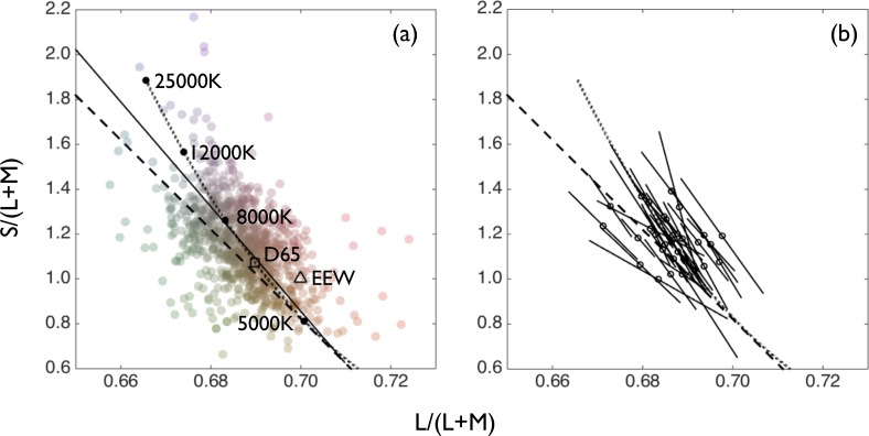
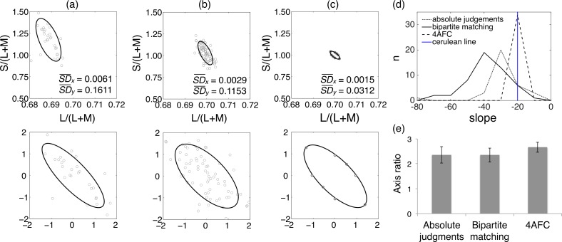
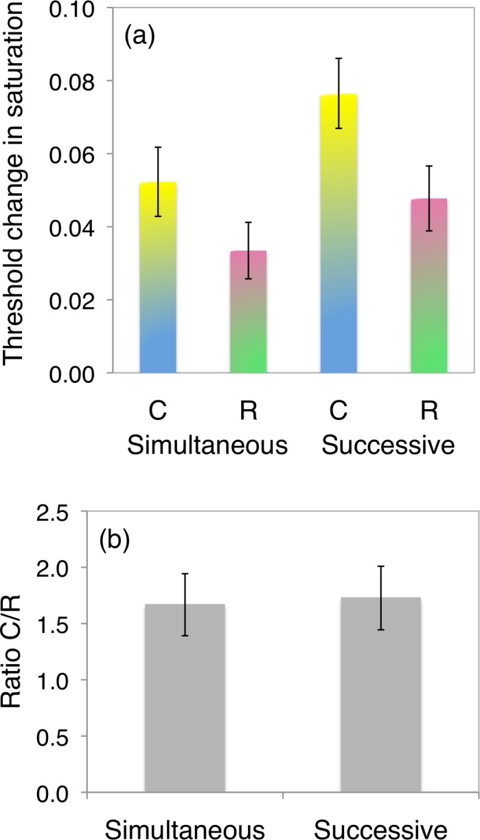
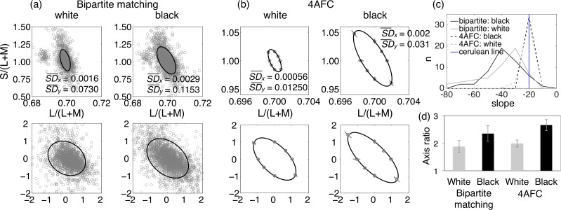
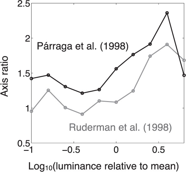
To shed light on the perceptual basis of the color white, we measured settings of unique white in a dark surround. We find that settings reliably show more variability in an oblique (blue-yellow) direction in color space than along the cardinal axes of the cone-opponent mechanisms. This is against the idea that white perception arises at the null point of the cone-opponent mechanisms, but one alternative possibility is that it occurs through calibration to the visual environment. We found that the locus of maximum variability in settings lies close to the locus of natural daylights, suggesting that variability may result from uncertainty about the color of the illuminant. We tested this by manipulating uncertainty. First, we altered the extent to which the task was absolute (requiring knowledge of the illumination) or relative. We found no clear effect of this factor on the reduction in sensitivity in the blue-yellow direction. Second, we provided a white surround as a cue to the illumination or left the surround dark. Sensitivity was selectively worse in the blue-yellow direction when the surround was black than when it was white. Our results can be functionally related to the statistics of natural images, where a greater blue-yellow dispersion is characteristic of both reflectances (where anisotropy is weak) and illuminants (where it is very pronounced). Mechanistically, the results could suggest a neural signal responsive to deviations from the blue-yellow locus or an adaptively matched range of contrast response functions for signals that encode different directions in color space.

Figure 1

Settings of absolute white from all participants. (a) Each data point represents one setting for one participant. The dashed line is the cerulean line. The dotted line is the locus of CIE daylights. The continuous black line is the orthogonal linear regression through the data. The locations of equal-energy white (EEW), D65, and CIE daylights of particular (labeled) color temperatures are marked. Two outlying data points of S/(L+M) > 2.2 do not appear on this plot. (b) For each participant, the mean white setting is indicated by a circle and the axis of maximum variability by a continuous black line. The line subtends one standard deviation on either side of the mean.

Figure 2

Results of Experiment 2. (a–c) Example data from a single participant for each of the three tasks. The standard deviations of the L/(L+M) (x) and the S/(L+M) (y) data points are provided on each plot. (a, left) Judgments of absolute white made in Experiment 1. (b, left center) Bipartite matches. (c, right center) Four-alternative forced-choice color discrimination. In each case, data are shown in the MacLeod-Boynton chromaticity diagram in the upper panel. For absolute judgments and for bipartite matching, the fitted ellipses are standard deviation ellipses. For four-alternative forced choice, they are fit through the eight data points measured. In each case, the fitting is done in a version of the MacLeod-Boynton chromaticity diagram that is transformed so that variability along the x and y axes is equal. The ellipses are transformed back for plotting in the original spaces. The lower panels show the data and fitted ellipses in the transformed MacLeod-Boynton chromaticity diagrams. (d, top right) Distributions of the slopes of the major axes of the ellipses. The slope of the cerulean lines is shown for comparison. (e, bottom right) Comparison of axis ratios for Experiments 1 and 2. The axis ratios are not significantly different between the three conditions.

Figure 3

Results of Experiment 3. (a) Average threshold for detection of a change in saturation in our two conditions, successive discrimination and simultaneous discrimination. The saturation scale s can be converted to our MacLeod-Boynton coordinates by S/(L+M) = s*cos(d) and L/(L+M) = 0.0623s*sin(d), where d = 141 or 321 for the cerulean line and d = 39 or 219 for the reflection. In both simultaneous and successive conditions, thresholds are significantly higher along the cerulean line (C) than along the reflection of the cerulean line (R). However, when the ratio of thresholds along the cerulean line to thresholds along the reflection is taken, there is no significant difference between conditions (b).

Figure 4

Results of Experiment 4. (a) Standard deviation ellipses fit to data combined from all participants for the bipartite matching task. The left panels show matches on the white surround, and the right panels show matches on the black surround. In the upper panels, the data are shown in the MacLeod-Boynton chromaticity diagram, and in the lower panels, they are shown in our transformed space. (b) Discrimination ellipses averaged across all participants for the four-alternative forced-choice task. The four subplots are equivalent to those in (a). Error bars indicate 95% confidence intervals. On the upper plots of (a) and (b), the standard deviations of the L/(L+M) (x) and the S/(L+M) (y) data points are provided. (c) Distributions of the slopes of the major axes of the ellipses for all subjects in all conditions. The slope of the cerulean line is shown for comparison. (d) Axis ratios for all conditions. For both bipartite matching and for four-alternative forced choice, axis ratios are significantly greater for the black surround than for the white surround. Error bars indicate 95% confidence intervals.

Figure 5

Axis ratios for the distributions of chromaticities in natural scenes. (a) The mean axis ratios for five sets of hyperspectral images of visual scenes are shown by the gray bars, compared with a summary of the axis ratios from Experiments 1, 2, and 4 by the blue bars. Error bars are 95% confidence intervals. (b) Distribution of axis ratios for all hyperspectral images of visual scenes.

Figure 6

Variation of axis ratio with luminance in the data of Párraga et al. (1998) and of Ruderman et al. (1998).

References

1. Abramov, I.,, Gordon J. (1994). Color appearance: on seeing red—or yellow, or green, or blue. Annual Review of Psychology, 45, 451–485. - PubMed
1. Ayama M.,, Nakatsue T.,, Kaiser P. K. (1987). Constant hue loci of unique and binary balanced hues at 10, 100, and 1000 Td. Journal of the Optical Society of America. A, Optics and Image Science, 4, 1136–1144. - PubMed
1. Beer D.,, Wortman J.,, Horwits G.,, MacLeod D. (2005). Compensation of white for macular pigment filtering. Journal of Vision, 5 (8): 5 doi:10.1167/5.8.282 [Abstract]
1. Berlin B.,, Kay P. (1969). Basic color terms: Their universality and evolution. Berkeley: University of California Press.
1. Bosten J.,, Lawrance-Owen A. (2014). No difference in variability of unique hue selections and binary hue selections. Journal of the Optical Society of America. A, Optics, Image Science, and Vision, 31, A357–A364. - PubMed
Publication types