Neural Coding of Perceived Odor Intensity

Abstract

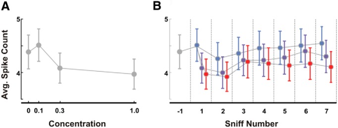
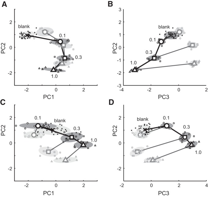
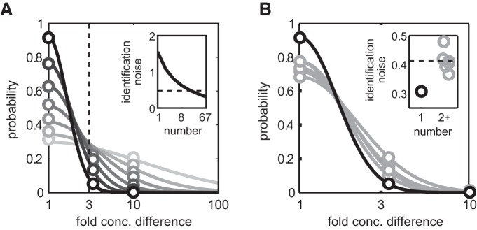
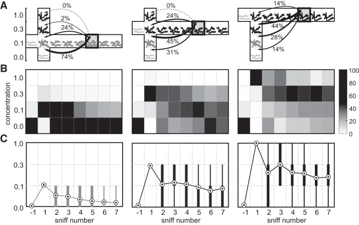
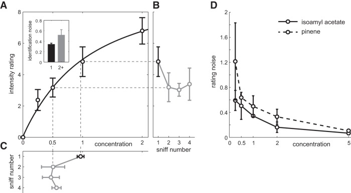
Stimulus intensity is a fundamental perceptual feature in all sensory systems. In olfaction, perceived odor intensity depends on at least two variables: odor concentration; and duration of the odor exposure or adaptation. To examine how neural activity at early stages of the olfactory system represents features relevant to intensity perception, we studied the responses of mitral/tufted cells (MTCs) while manipulating odor concentration and exposure duration. Temporal profiles of MTC responses to odors changed both as a function of concentration and with adaptation. However, despite the complexity of these responses, adaptation and concentration dependencies behaved similarly. These similarities were visualized by principal component analysis of average population responses and were quantified by discriminant analysis in a trial-by-trial manner. The qualitative functional dependencies of neuronal responses paralleled psychophysics results in humans. We suggest that temporal patterns of MTC responses in the olfactory bulb contribute to an internal perceptual variable: odor intensity.

Keywords: Concentration versus adaptation; extracellular electrophysiology; human psychophysics; olfactory bulb.

Figure 1.

MTC responses change with odor concentration. A, Sniff-warped raster and PSTH plots of sharp excitatory (I-cyan), excitatory (II-brown), and inhibitory (III-green) responses of individual MTCs for 3-fold and 10-fold changes in odor concentration (shown as color shades). Top, Schematic sniff waveform. Gray shading, Inhalation; gray trace, activity of the MTC during blank sniffs. Vertical dashed lines indicate the beginning and end of inhalation interval. B, Distribution of different response types observed in the data. C, Scatter plot comparing amplitude and latency of sharp, excitatory and inhibitory responses (color notations as in B). Boxplots show marginal response distributions: circle is median, thick line is the IQR, thin lines on either side extend to 1.5 × IQR beyond the 25% and 75% quartiles or the farthest data point, whichever is smaller. D, Normalized distributions of changes of latencies (left column), amplitude (central column), and firing rate (right column) with a threefold concentration change across cells for different response types (color notations as in B). Colored asterisks denote significance of test for zero median (*p < 0.05, **p < 0.01, ***p < 0.001; Wilcoxon rank sum test). Black solid and dashed lines show distributions of response latencies for early (<100 ms) and late (>100 ms) responses respectively. Black asterisks denote significant differences between two distributions. Arrows mark the position of the median.

Figure 2.

A, Latency of the first spike estimated using distributions of interspike intervals (Shusterman et al., 2011) for responses identified as sharp pooled across all odors and concentrations versus the latency of the peak PSTH for the same response. B, Difference in absolute PSTH latency between sharp responses to high and 3× lower concentrations versus the relative latency estimated using cross-correlation (see Materials and Methods).

Figure 3.

MTC responses change with repeated sampling. A, Sniff-warped raster and PSTH plots of sharp excitatory (I), excitatory (II), and inhibitory (III) responses of single MTCs during the first, fourth, and seventh sniff cycles (shown as color shades). A schematic of the sniff waveform is shown above the plots. Gray shading and vertical dashed lines delineate inhalation period. Gray trace, Activity of the mitral/tufted cell during unodorized sniffs. B, Scatter plot comparing amplitude and latency of excitatory, sharp, and inhibitory responses on the seventh sniff following odor onset. Boxplots show marginal response distributions, as in Figure 1C . Color conventions as in Figure 1. C, Colored lines are normalized distributions of changes in latency, amplitude, and firing rate of sharp, excitatory, and inhibitory responses with adaptation (difference between first and seventh sniffs). Black solid and dashed lines are the same distributions for early and late responses. Notations are same as in Figure 1D .

Figure 4.

Correlated changes in response features for concentration and adaptation. From left to right, plots show changes in the latency, amplitude, and mean firing rate. Points are individual response sets. Response types are indicated by color as in Figure 1. Box plots show distributions of response changes across cells for concentration and adaptation. Conventions are as in Figure 1. Reported r values are Spearman correlation coefficients computed independently for the three response types. Black arrows mark positions of the three example cells in Figures 1 and 2.

Figure 5.

Spike count unlikely to code odor intensity. A, Average number of spikes observed on a single sniff for each unit as a function of odor concentration. B, Average number of spikes per sniff per cell observed on each sniff for the three tested concentrations and baseline (gray, baseline; light blue, 0.1; dark blue, 0.3; red, 1.0). Error bars indicate the SD across trials.

Figure 6.

Principal component analysis of the population vector changes with concentration and adaptation. A, B, The full temporal population vectors plotted in the space of the first and second (A) and second and third (B) principal components. Large symbols, Average PC projection of all first sniffs (black) and seventh sniffs (gray); small symbols, projection of 10 independent subsets of the full dataset (shaded ovals, SD). Blank is cross symbol; concentration 0.1, 0.3, and 1.0, respectively, are circles, squares, and triangles. Black lines connect first sniffs of different concentrations. Gray lines connect first and seventh sniffs of the same concentration. Numbers denote the presented concentrations. C, D, Same as A and B, but for average firing rate population vector.

Figure 7.

Adaptation increases concentration identification error. A, Results of classification analysis for concentration discrimination between four levels (0.0, 0.1, 0.3, 1.0): average probability of classification (empty circles) of temporal patterns of MTCs at the first sniff as a function of concentration mismatch between actual concentration and classified concentration (1 corresponds to correct classification, 3(10) is the classification mismatch for 1(2) step threefold concentration differences) for different numbers of cells (shading from lightest to darkest corresponds to 1, 2, 4, 8, 16, 32, and 67 cells). Solid lines are Gaussian fits of classification probability: $p=p_1\mathrm{e}\mathrm{x}\mathrm{p}\left(-{\left(\Delta {\mathrm{l}\mathrm{o}\mathrm{g}}_{10}\left(\mathrm{C}\right)\right)}^2/{\mathrm{\sigma }}^2\right)$, where p1 is a probability of correct classification, and σ is the concentration classification error in log10 units. Inset, Concentration classification error as a function of number of cells included in classification. Vertical dashed line: threefold concentration difference. B, Classification performance for all 67 cells for different sniffs following odor onset (black, sniff 1; gray, sniffs 2-7). Inset: concentration classification error for sniff 1 (black) vs later sniffs (gray). Dashed line: median for sniffs 2+.

Figure 8.

Adaptation decreases the encoded odor concentration. Single-trial responses were classified based on their Euclidean distance to the average responses to the three concentrations presented on the first sniff and the average blank response. A, Schematics of the classification process for three concentrations (left, 0.1; middle, 0.3; right, 1.0). Responses on a given sniff and concentration (examples are shown in boxes) are classified against responses on the first sniff. The arrows from sniff 5 (shaded box) illustrate match probabilities between this sniff and responses on the first sniff. B, For each concentration (left to right), grayscale plots show the classifier match probability (see bar on right) for responses on a given sniff (x-axis) with the average concentration responses on the first sniff (y-axis). C, Equivalent concentration for each sniff calculated as the average match probability weighted by concentration (circles), and distributions of classification results: thin line is the 10-90% interval; and thick lines are the 25-75% interval.

Figure 9.

Effect of adaptation on perceived odor intensity. A, Average intensity ratings for different concentrations of the odor pinene obtained on the first sniff (black) and after adaptation (gray). Curve denotes average Hill equation fit between concentration and perceived intensity. Concentration has been normalized such that concentration 1 corresponds to 60 ml/min saturated vapor diluted in a typical 2 s inhalation and a peak flow rate of 50 L/min (minimum 0.12% saturated vapor). Inset, Rating noise (rating SD/mean). B, Perceived intensity of the odor stimulus with concentration 1 across sniffs from a constant odor source. C, Equivalent concentration computed as the concentration with the same intensity rating on the first sniff extrapolated from the Hill equation fit for individual subjects (schematized by dashed gray lines). Error bars indicate the SD across subjects included in the analysis. D, Rating noise as a function of presented odor concentration for pinene (dashed) and isoamyl acetate (solid).

References

1. Abraham NM, Spors H, Carleton A, Margrie TW, Kuner T, Schaefer AT (2004) Maintaining accuracy at the expense of speed: stimulus similarity defines odor discrimination time in mice. Neuron 44:865–876. 10.1016/j.neuron.2004.11.017 - DOI - PubMed
1. Anderson AK, Christoff K, Stappen I, Panitz D, Ghahremani DG, Glover G, Gabrieli JDE, Sobel N (2003) Dissociated neural representations of intensity and valence in human olfaction. Nat Neurosci 6:196–202. 10.1038/nn1001 - DOI - PubMed
1. Bathellier B, Buhl DL, Accolla R, Carleton A (2008) Dynamic ensemble odor coding in the mammalian olfactory bulb: sensory information at different timescales. Neuron 57:586–598. 10.1016/j.neuron.2008.02.011 - DOI - PubMed
1. Beck A, Kruger L, Calabresi P (1954) Observations on olfactory intensity. I. Training procedure, methods, and data for two aliphatic homologous series. Ann N Y Acad Sci 58:225–238. - PubMed
1. Bodyak N, Slotnick B (1999) Performance of mice in an automated olfactometer: odor detection, discrimination and odor memory. Chem Senses 24:637–645. - PubMed
Publication types
LinkOut - more resources