Isotonic Regression Based-Method in Quantitative High-Throughput Screenings for Genotoxicity

Abstract

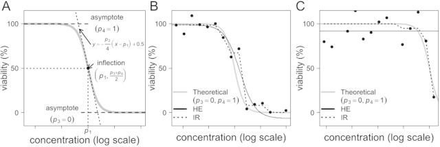
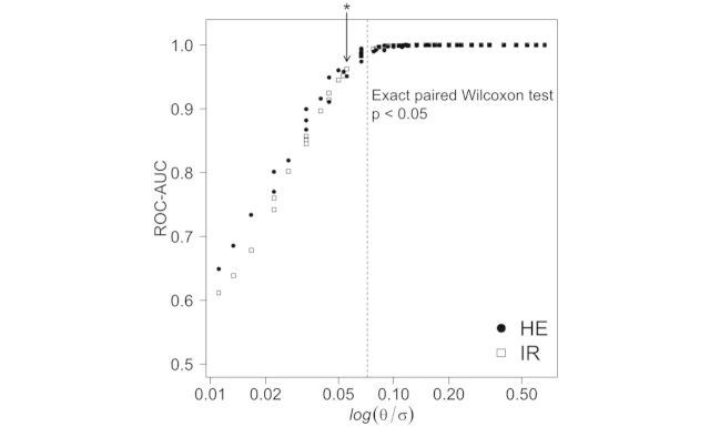
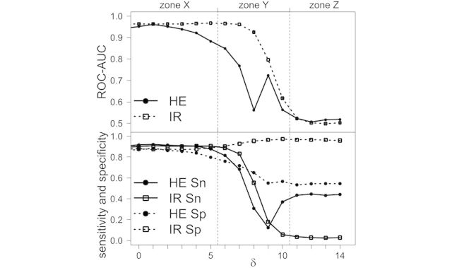
Quantitative high-throughput screenings (qHTSs) for genotoxicity are conducted as part of comprehensive toxicology screening projects. The most widely used method is to compare the dose-response data of a wild-type and DNA repair gene knockout mutants, using model-fitting to the Hill equation (HE). However, this method performs poorly when the observed viability does not fit the equation well, as frequently happens in qHTS. More capable methods must be developed for qHTS where large data variations are unavoidable. In this study, we applied an isotonic regression (IR) method and compared its performance with HE under multiple data conditions. When dose-response data were suitable to draw HE curves with upper and lower asymptotes and experimental random errors were small, HE was better than IR, but when random errors were big, there was no difference between HE and IR. However, when the drawn curves did not have two asymptotes, IR showed better performance (p < 0.05, exact paired Wilcoxon test) with higher specificity (65% in HE vs. 96% in IR). In summary, IR performed similarly to HE when dose-response data were optimal, whereas IR clearly performed better in suboptimal conditions. These findings indicate that IR would be useful in qHTS for comparing dose-response data.

Keywords: Hill equation; Isotonic regression; genotoxicity; quantitative high-throughput screening.

FIGURE 1.

Theoretical and estimated dose-response curves and classification of estimated curves.(A) The theoretical HE curve has two asymptotes at 0 (0%) and 1 (100%) viabilities, and the inflectionin the middle of the slope. The y-coordinates of the two asymptotes, the coordinates of the inflection,and the equation of the tangent line at the inflection, are indicated using the parameters in equation (1). (B) When observing concentrations covered by the range including the two asymptotes, the HE estimation curve (solid line) had two asymptotes and an inflection, so the estimated curve was called “complete” based on the NCGC classification criteria. Both HE and IR estimation curves (solid and dotted, respectively) were close to the theoretical curve (grey). Only one curve is drawn for simplicity. (C) On the other hand, when observing concentrations that only partially covered the range, the HE estimation curve had only one asymptote with an inflection, and the estimated curve was called “incomplete” based on the criteria. The estimated IR curve (dotted) had only one asymptote as well, but it fit better to the theoretical curve than the HE curve.

FIGURE 2.

Simulation designs. (A) For the theoretical dose-response curves, we fixed two parameters, p₃ and p₄, out of the four parameters in equation (1) and rewrote equation (2) with two parameters, a = p₁ and b = p₂. The viability was a function of concentration provided on a logarithmic scale. When the compound was a typical genotoxicant via the mutated gene function, the two doseresponse curves of wild-type (solid) and mutant (dotted) were parallel with a horizontal shift. The horizontal shift of the mutant line to the left meant that the mutant cells were less viable as lower concentrations of the compound. The effect size of the genotoxicity was defined as the horizontal shift, θ = a_w - a_m, which is indicated as “Effect size” on the graph. The experimentally observed viabilities deviated from the curve with random errors, as indicated by filled circles (wild-type) and rectangles (mutant). Random errors are indicated by a box plot in the panel. This dataset was generated with θ / σ = 0.167. (B) This plot describes suboptimal conditions where the experimental concentrations did not cover the dose-response curves well. When the coverage was suboptimal, the estimated curve did not have two asymptotes and it was classified as “incomplete”. The parameter δ controlled the location of the experimental concentrations relative to the theoretical curves. Each dotted rectangle corresponds to δ = 0, 8, and 14 as it shifts to the left. We observed cell viability from the minimum concentration to the maximum concentration for each simulation. Zone X, Y, and Z are described in Figure 5. (C) This panel describes a compound whose dose-response curves in wild-type and mutant were not parallel and had an intersection in the middle of the slopes. This indicated that the compound had a greater effect lowering the viability of the mutant cells when its concentration was low, but when its concentration was high, the viability of wild-type cells was lower. Although it is not easy to explain this phenomenon by simple biological models, the estimated curves based on observation sometimes fit this pattern. (D) This panel describes how υ changed the shapes of curves. When υ = 0, the wild-type and mutant curves were parallel, but when υ > 0, the slope of the mutant curve was steeper, and when υ < 0, the slope of the wild-type curve was steeper. The two mutant curves represented the largest and smallest υ from -3 to 1, which was the range we evaluated in this report.

FIGURE 3.

The estimated curves obtained using the Hill equation and isotonic regression methods, wand the statistics for the genotoxicity results. (A) The filled circles and rectangles represent observed viability values for the wild-type and mutant cell lines, respectively. Two curves were estimated with HE. The solid curve is of the wild-type cell line and the dotted curve is of the mutant cell line. The statistics for the genotoxicity results, ΔS_HE, is the distance between the horizontal coordinates of p₁ (log₁₀EC⁵⁰) of the two curves. (B) For the same dataset, isotonic regression (IR) provided two lines, the wild-type line (solid) and the mutant line (dotted). The points g_w(x) are on the solid line and the points g_m(x) are on the dotted line. Both solid and dotted lines decreased monotonically, and the solid line was above the dotted line throughout. Four inequality restrictions for x₁₀ and x₁₁ are indicated. The statistics for the genotoxicity results, indicated. The statistics for the genotoxicity results, ΔS_IR, is the area between two lines, which is shadowed.

FIGURE 4.

The relationship between θ / σ and ROC-AUC. When the ratio of the true effect sizes to the variance of the random errors was smaller than the vertical dotted line (the left side of Figure), the ROC-AUC of HE was better than that of IR. On the other right side, the performance of the two methods was not different. The two methods were tested for differences for all θ / σ values as a set, which was statistically significant (p < 0.05, exact paired Wilcoxon test). The majority of θ / σ on the left side were also significant when compared individually (p < 0.05, DeLong test). The vertical dotted line corresponds to θ / σ = 0.067. The asterisk The asterisk (*) and an arrow indicate θ / σ = 0.056, used in the data generation of Figure 5 (σ = 18, θ = 1).

FIGURE 5.

ROC-AUC (top), and sensitivity and specificity (bottom) with various δ, with σ = 18, θ = 1 and υ = 0. θ / σ of this experiment is provided in Figure 4. δs were divided into 3 zones, Zone X, Y, and Z, as described in the main text. (Top) In zone X, both methods had similar performance, but HE was more subject to δ. In zone Y, the reliability of both methods decreased, but the decrease in HE was more rapid than that of IR. In zone Z, both ROC-AUCs were 0.5. (Bottom) Sensitivity and specificity. In zone Z, the sensitivity and specificity of HE were 0.5, while the sensitivity and specificity of IR were almost 0 and 1, respectively. Both plots share the horizontal axis δ Abbreviations: Sn = sensitivity, Sp = specificity

FIGURE 6.

The effect of vn on the statistics of HE and IR (A) When dose-survival curves of the wildtype and the mutant were parallel (υ = 0), the area between the two curves was identical to θ = a_w - a_m, indicated as a grey rectangle. (B) When the two curves were not parallel (υ ≠ 0), the area between the two curves was divided into S⁺ and S^-. In this case, the area was also identical to θ = a_w - a_m, namely, ΔS_HE. (C) IR estimated the area S^- to be zero because of the restriction of g_w(x_i) ≥ g_m(x_i). (D) The effect of υ on ΔS_HE and ΔS_IR. The ratio of ΔS_* (*: HE, IR) to ΔS_* at υ = 0 was plotted. υ did not affect ΔS_HE while it affected ΔS_IR. (E) The relationship between θ / σ and ROC-AUC at υ = 1. In contrast to Figure 4, the overall ROC-AUC of IR was better than that of HE (p < 0.05, exact paired Wilcoxon test) and the majority of θ / σ on the left side were also significant when compared individually (p < 0.05, DeLong test).

FIGURE S1.

The area between the wild-type and mutant curves. (A) When the two curves are parallel, the area is indicated as a grey area. This is identical to the grey rectangle whose width is θ = a_w - a_m, located at the right side of the Figure. (B) When the two curves intersected, the area was divided into S⁺ where the wild-type curve was higher than the mutant curve, and S^- where the wild-type curve was lower than the mutant curve. Area S⁺ corresponds to the mesh triangle and area S^- corresponds to the dark grey triangle. S^- has a negative value, but S⁺ increased by the same amount as S^-. That is, S⁺ + S^- is identical to θ = ΔS_HE (light grey rectangle). (C) One of the restrictions of IR, that the line for the wildtype should not be below the line for the mutant, made the area S^- zero. S^- is shown as a dark grey triangle in Figure S1B, while here, S^- is indicated as a line. That is, ΔS_IR = S⁺ is larger than θ = ΔS_HE.

FIGURE S2.

Calculation of the statistics for isotonic regression (IR) via the trapezoidal rule. The grey area under the dashed lines after IR estimation, S_i, was calculated by the trapezoidal rule and summed through to iteration i. The two parallel bases and the height correspond to g(x_i), g(x_i+1), and log₁₀r, respectively.

References

1. Best MJ, Chakravarti N. 1990. Active set algorithms for isotonic regression; a unifying framework. Mathematical Programming 47:425–39.
1. Byrd RH, Byrd RH, Lu P, Lu P, Nocedal J, Nocedal J, Zhu C. 1994. A limited memory algorithm for bound constrained optimization. SIAM Journal on Scientific Computing 16:1190–208.
1. Collins FS, Gray GM, Bucher JR. 2008. Toxicology. transforming environmental health protection. Science 319(5865):906–7. - PMC - PubMed
1. DeLong ER, DeLong DM, Clarke-Pearson DL. 1988. Comparing the areas under two or more correlated receiver operating characteristic curves: A nonparametric approach. Biometrics Sep(44(3)):837–45. - PubMed
1. Evans TJ, Yamamoto KN, Hirota K, Takeda S. 2010. Mutant cells defective in DNA repair pathways provide a sensitive high-throughput assay for genotoxicity. DNA Repair (12):1292–8. - PubMed