Mapping Sub-Second Structure in Mouse Behavior

Abstract

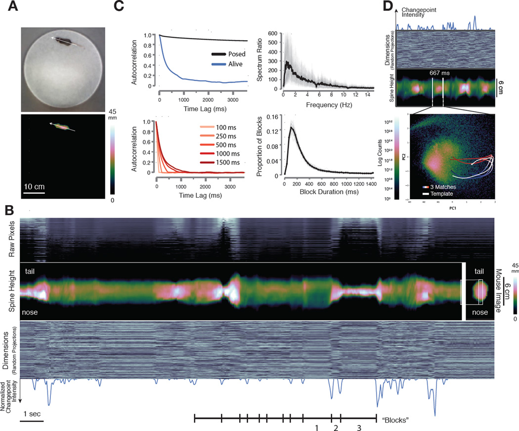
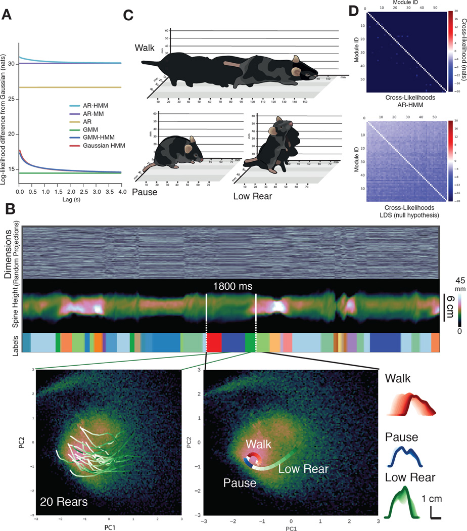
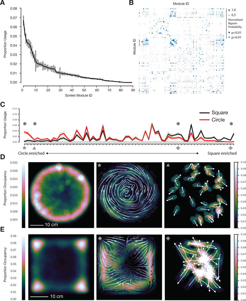
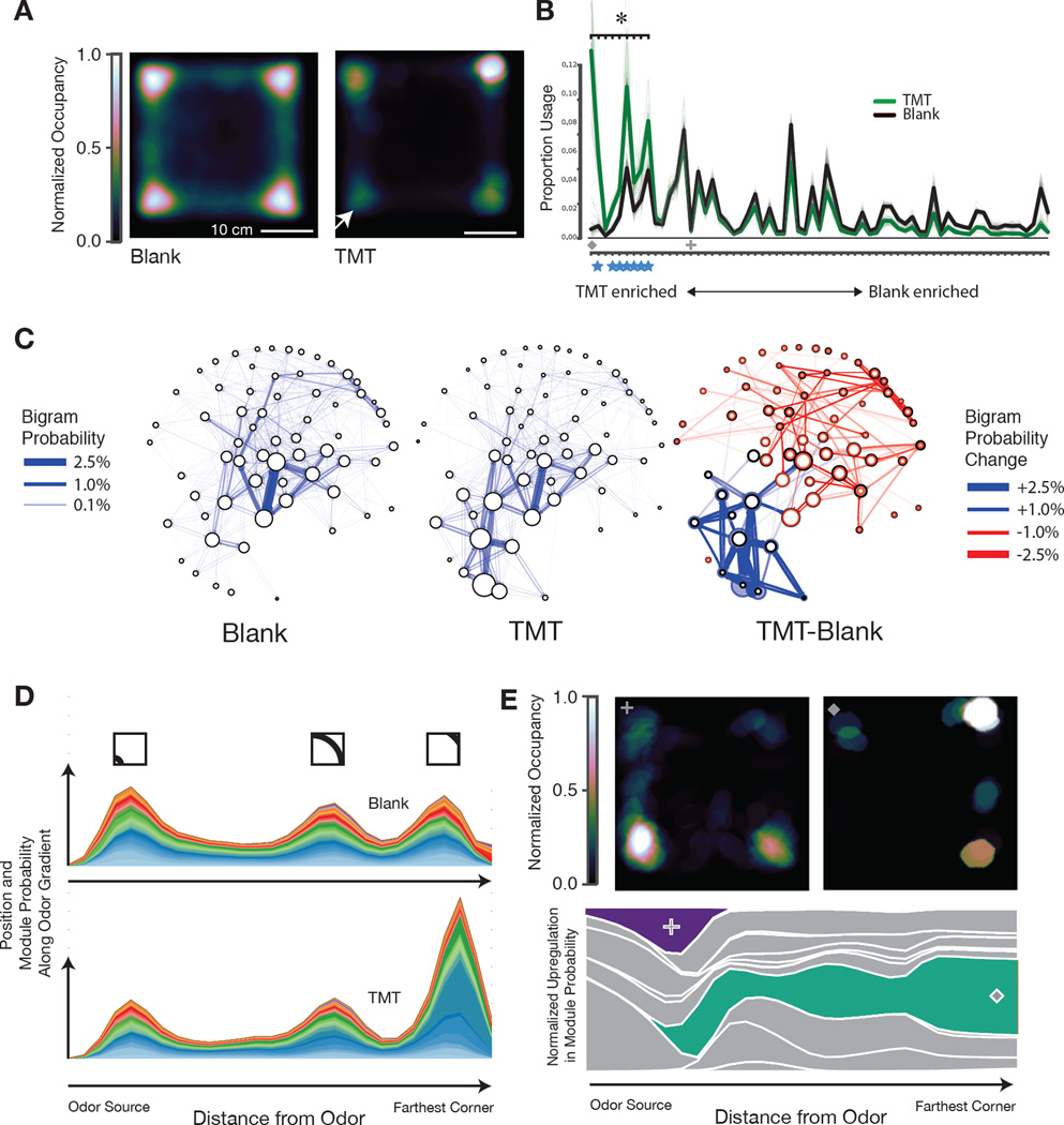
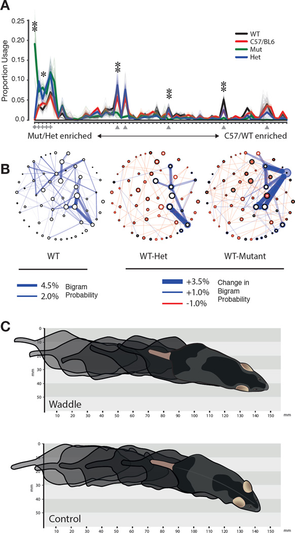
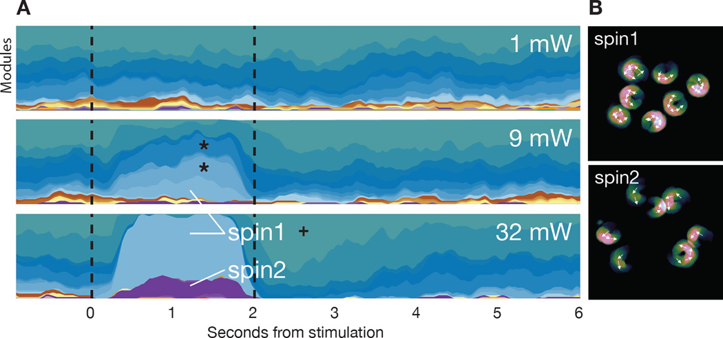
Complex animal behaviors are likely built from simpler modules, but their systematic identification in mammals remains a significant challenge. Here we use depth imaging to show that 3D mouse pose dynamics are structured at the sub-second timescale. Computational modeling of these fast dynamics effectively describes mouse behavior as a series of reused and stereotyped modules with defined transition probabilities. We demonstrate this combined 3D imaging and machine learning method can be used to unmask potential strategies employed by the brain to adapt to the environment, to capture both predicted and previously hidden phenotypes caused by genetic or neural manipulations, and to systematically expose the global structure of behavior within an experiment. This work reveals that mouse body language is built from identifiable components and is organized in a predictable fashion; deciphering this language establishes an objective framework for characterizing the influence of environmental cues, genes and neural activity on behavior.

Fig. 1. Depth imaging reveals block structure in 3D mouse pose dynamics data

A. Mouse imaged in the circular open field with a standard RGB (top) and 3D depth camera (bottom, mm = mm above floor). Arrow indicates the inferred axis of the animal’s spine. B. Raw pixels of the extracted and aligned 3D mouse image (top panel, sorted by mean height), compressed data (bottom panel, 300 dimensions compressed via random projections arrayed on the Y axis, pixel brightness proportional to its value), and height at each inferred position of the mouse’s spine (middle panel, “spine” data extracted from the mouse as indicated on the right, mm = mm above floor) each reveal sporadic, sharp transitions in the pose data over time. Note that the cross-sectional profile of the spine with respect to the camera varies depending upon the morphology of the mouse; when reared this profile becomes smaller, and when on all fours it becomes larger. Changepoints analysis (bottom panel, blue trace = normalized changepoint probability) identifies approximate boundaries between blocks. Blocks encode a variety of behaviors including locomotion (1), a pointing rear with the mouse’s body elongated with respect to the sensor (2), and a true rear (3). C, upper left. Autocorrelation analysis performed on the top 10 dimensions of principal components data reveals that temporal correlation in the mouse’s pose stabilizes after about 400 milliseconds (tau = 340 ± 58 ms). C, lower left. Shuffling behavioral data in blocks of 500 milliseconds or shorter destroys autocorrelation structure (shuffle block size indicated). C, upper right. Spectral power ratio between a behaving and dead mouse (mean plotted in black, individual mice plotted in grey) reveals most frequency content is represented between 1 and 6 Hz (mean = 3.75 ± .56 Hz). C, lower right. Changepoints-identified block duration distribution (mean = 358 ms, SD 495 ms, mean plotted in black, individual mice in gray, n=25 mice, 500 total minutes imaging,). D. Projecting mouse pose data (top panels, random projections and spine data depicted as in B) into Principal Component (PC) space (bottom) reveals that blocks of pose data encode reused trajectories (density of all recorded poses colormapped behind trajectories). Tracing out the path associated with a block highlighted by changepoint detection (top) identifies a trajectory through PC space (white). Similar trajectories identified through template matching (time indicated as progression from blue to red), are superimposed. Note that this procedure uses the first 10 PCs to identify matched trajectories, although only the first two PCs are depicted here.

Fig. 2. Reused behavioral modules within mouse pose dynamics data

A. Predictive performance comparison of computational models describing possible structures for behavior (details of each model and the comparison metric provided in Supplemental Experimental Procedures). Models range from a Gaussian model (which proposes that mouse behavior is built from modules, each a single Gaussian in pose space) to an AR-HMM (which proposes that mouse behavior is built from modules, each of which encodes an autoregressive trajectory through pose space, and which transition from one to another with definable transition statistics; AR-MM = autoregressive mixture model, AR = autoregressive model, GMM = Gaussian mixture model, GMM-HMM = GMM hidden Markov model, Gaussian HMM = Gaussian hidden Markov model). Model performance plotted as the log likelihood (Y-axis) ascribed to held-out test data at some time lag (X-axis) into the future (after subtracting Gaussian model performance). B. The AR-HMM parses behavioral data into identifiable modules (top panels – marked “labels”, each module is uniquely color coded). Multiple data instances associated with a single behavioral module (between green lines, encoding a rear) each take a stereotyped trajectory through PC space (bottom left, trajectories progress from white to green over time, see Movie S4); multiple trajectories define behavioral sequences (bottom center, see Movie S6). Each trajectory within a sequence encodes a different elemental action (side-on view of the mouse calculated from depth data, bottom right, time indicated as increasingly darker lines, from module start to end). C. Isometric-view illustrations of the 3D imaging data associated with walk, pause and low rear modules (also see Movie S4). D. Cross-likelihood analysis depicting the likelihood that a data instance assigned to a particular module is well-modeled by another module. Cross-likelihoods were computed for the open field dataset (above, see Supplemental Experimental Procedures, units are nats, where e^nats is the likelihood ratio) and for module-free synthetic data whose autocorrelation structure matches actual mouse data (below).

Fig. 3. The physical environment influences module usage and spatial pattern of expression

A. Modules identified by the AR-HMM, sorted by usage (n = 25 mice, 20 minutes per mouse, data from circular open field, error bars are SEs calculated using bootstrap estimation, n=100 bootstrap estimates, see Fig. S5E for Bayesian credible intervals). B. Hinton diagram depicting the probability that any pair of modules is observed as an ordered pair (p-values calculated via bootstrap estimation and color coded); modules were sorted by spectral clustering to emphasize neighborhood structure. C. Module usage, sorted by context (with “circleness” on left, overall usages differ significantly, p < 10⁻¹⁵, Hotelling two-sample t-squared test, see Supplemental Experimental Procedures for sorting details). Mean usages across animals depicted with dark lines, with bootstrap estimates depicted in fainter lines (n=100). Marked modules discussed in main text and shown in panel D: star = circular wall-hugging locomotion (“thigmotaxis”), triangle = outward-facing rears, diamond = square thigmotaxis, cross = square dart, see Movie S7. Usage for all marked modules significantly modulated by context (indicated by asterisk, Wald Test, Holm-Bonferroni adjusted p < 0.006 for square dart, otherwise p < 10⁻⁵). D. Occupancy plot of mice in circular open field (left, n=25, 500 minutes total) indicating cumulative spatial positions across all experiments. Occupancy plot depicting deployment of circular thigmotaxis module (middle, average orientation across the experiment indicated as arrow field) and circle-enriched outward-facing rear module (right, orientation of individual animals indicated with arrows). E. Occupancy plot of mice in square box (left, n=15, 300 minutes total) indicating cumulative spatial positions across all experiments. Occupancy plot depicting a square-enriched thigmotaxis module (middle, average orientation across the experiment indicated as arrow field), and square-specific darting module (right, orientation of individual animals indicated with arrows).

Fig. 4. Odor-driven innate avoidance alters transition probabilities

A. Occupancy plot of mice under control conditions (n=24, 480 minutes total) and after exposure to the fox-derived odorant trimethylthiazoline (TMT, 5% dilution, n=15, 300 minutes total, model co-trained on both conditions) in the lower left quadrant (arrow). Plots normalized such that maximum occupancy = 1. B. Module usage plot sorted by “TMT-ness” (Dark lines depict mean usages, bootstrap estimates depicted in fainter lines, sorting as in Fig. 3). Marked modules discussed in main text and panel E: cross = sniff in TMT quadrant, diamond = freeze away from TMT, see Movies S8 and S9. Blue stars indicate freezing modules. Asterisk indicates statistically-significant regulation (Wald test, Holm-Bonferroni corrected, p < 10⁻⁴). C, left and middle. Behavioral state maps for mice exploring a square box before and after TMT exposure, with modules depicted as nodes (usage proportional to the diameter of each node), and bigram transition probabilities depicted as directional edges. Graph layout minimizes the length of edges and is seeded by spectral clustering to emphasize local structure. C, right. Statemap depiction of the difference between blank and TMT. Usage differences are indicated by the newly-sized colored circles (upregulation indicated in blue, downregulation indicated in red, previous usages in control conditions indicated in black). Altered bigram transition probabilities are indicated in the same color code; only those significant transition probabilities (p<0.01) are depicted. D. Mountain plot depicting the joint probability of module expression and spatial position, plotted with respect to the TMT corner (X-axis); note that the “bump” two-thirds of the way across the graph occurs due to the two corners equidistant from the odor source (see inset for approximate position in square box, modules are color coded). E. Occupancy plot (upper) indicating spatial position at which mice after TMT exposure emit an investigatory sniffing module (left) or a pausing module (right, see Movie S8). Mountain plot (lower) indicating the differential deployment of these two modules (purple, green; other modules in grey) with respect to distance from the odor source.

Fig. 5. The AR-HMM disambiguates wild-type, heterozygous and homozygous Ror1β mice

A. Usage plot of modules exhibited by littermate Ror1β mice (n=25 C57/BL6, n = 3 +/+, n = 6 +/−, n = 4 −/−, open field assay, 20 minute trials), sorted by “mutant-ness” (sorting and depiction as in Fig. 3). Wild-type module usage is not statistically different from C57, but differs significantly from homozygote and heterozygote (Hotelling two-sample t-squared test, p < 10⁻¹⁵). Marked modules described in main text, diamond = waddle, triangle = normal locomotion, cross = pause. Single asterisk indicates significant usage difference between mutant and wildtype, p < 0.05, double asterisk indicates p < 0.01 under Wald test, Holm-Bonferroni corrected. B. State map depiction of baseline OFA behavior for +/+ animals as in Fig. 4C (left); difference state maps as in Fig. 4C between the +/+ and +/− genotype (middle), and +/+ and −/− genotype (right); all depicted transitions that distinguish genotypes are statistically significant, p<.01. C. Illustration of the “waddle” module in which the hind limbs of the animal are elevated during walking (see Movie S10).

Fig. 6. Optogenetic perturbation of motor cortex yields both neomorphic and physiological modules

A. Mountain plot depicting the probability of expression of each behavioral module (assigned a unique color on the Y axis) over time (X axis), with light stimulation indicated by dashed vertical lines (each plot is the average of 50 trials). Note that modest variations in the baseline pattern of behavior, due to trial structure, are captured before light onset. Stars indicate two modules expressed during baseline conditions that are also upregulated at intermediate powers (11 mW) but not high powers (32 mW, Wald test, Holm-Bonferroni adjusted p < 10⁻⁵); cross indicates pausing module upregulated at light offset (Wald test, Holm-Bonferroni adjusted, p < 10⁻⁵). B. Average position of example mice (with arrows indicating orientation over time) of the two modules induced under the highest stimulation conditions (see Movie S11). Note that A and B are generated from one animal and that the observed modulations are representative of the complete dataset (n= 4 mice, model was trained separately from previous experiments).

References

1. Aldridge JW, Berridge KC, Rosen AR. Basal ganglia neural mechanisms of natural movement sequences. Canadian Journal of Physiology and Pharmacology. 2004;82:732–739. - PubMed
1. Anderson DJ, Perona P. Toward a science of computational ethology. Neuron. 2014;84:18–31. - PubMed
1. André E, Conquet F, Steinmayr M, Stratton SC, Porciatti V, Becker-André M. Disruption of retinoid-related orphan receptor beta changes circadian behavior, causes retinal degeneration and leads to vacillans phenotype in mice. The EMBO journal. 1998;17:3867–3877. - PMC - PubMed
1. Berg HC, Brown DA. Chemotaxis in Escherichia coli analysed by three-dimensional tracking. Nature. 1972;239:500–504. - PubMed
1. Berman GJ, Choi DM, Bialek W, Shaevitz JW. Mapping the structure of drosophilid behavior. Journal of the Royal Society, Interface / the Royal Society. 2014;11:20140672. - PMC - PubMed
Publication types
LinkOut - more resources