Principles of cryo-EM single-particle image processing

Abstract

Single-particle reconstruction is the process by which 3D density maps are obtained from a set of low-dose cryo-EM images of individual macromolecules. This review considers the fundamental principles of this process and the steps in the overall workflow for single-particle image processing. Also considered are the limits that image signal-to-noise ratio places on resolution and the distinguishing of heterogeneous particle populations.

Keywords: 3D reconstruction; SNR; noise.

Fig. 1.

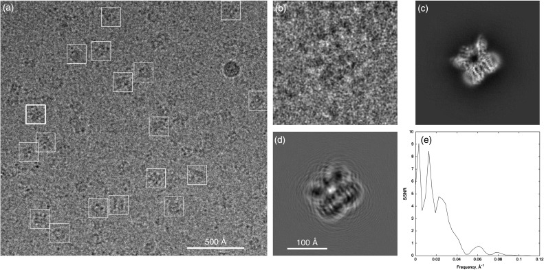
Cryo-EM micrograph and a particle image. (a) One quarter of a micrograph from the TRPV1 dataset of Liao et al. [6] with selected particles marked by boxes. (b), Boxed image (256 pixels on a side, pixel size 1.22 Å) of the particle marked with a thick box in (a). (c) Corresponding projection of the 3D map of the TRPV1 protein, computed according to the angles assigned to this particle image by the Relion reconstruction program [2]. TRPV1 is a membrane protein, here solubilized by amphipols, and the viewing direction is approximately in the membrane plane; the transmembrane region is at the lower right. (d) Simulated noiseless particle image, obtained by operating on the projection image with the fitted contrast-transfer function. Note the arcs extending from the particle due to signal delocalization from the substantial defocus δ = 2.2 µm. The electron wavelength is λ= 2 pm at 300 keV, and image features of characteristic size (resolution) d = 3.5 Å are expected to be delocalized by about λδ/d = 120 Å; hence the need for a large boxed image size. (e) Average particle spectral signal-to-noise ratio [7] computed from Fourier ring correlations between phase-flipped particle images and map projections. For display, images in (a) and (b) were Gaussian filtered with half power at 20 and 11 Å, respectively. Data are from micrograph 21 and particle image 4 in the EMPIAR database entry, http://dx.doi.org/10.6019/EMPIAR-10005.

Fig. 2.

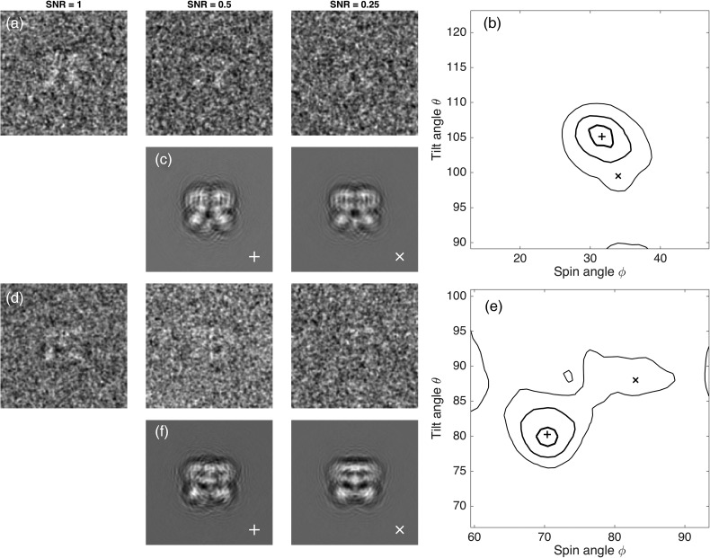
Angle assignment errors. Two particles from the micrograph in Fig. 1 were chosen as representative. They are approximately side views with tilt angles θ = 160° and 80° and spin angles $\varphi ={31}^{\circ }$ and 70°. Sets of 10 000 simulated particle images were computed with noise variance either matching that of the actual particles (labeled SNR = 1) or variance that is larger by a factor of 2 or 4, yielding the relative SNR values of 0.5 or 0.25. In rows (a) and (d), images with reversed contrast (protein is white) are shown after Gaussian filtering at 15 Å. Orientation angles were obtained by projection-matching for each image. (b and e) Contours enclosing 50% of the estimated angle values are shown for the two particles at three SNR values. In each plot, the thickest contour line corresponds to SNR = 1, where the standard deviation of errors in both angles was 1.7°. At SNR = 0.5, the errors had a standard deviation of 3° while at SNR = 0.25 angle errors of 10° or more were common, as shown by the thin contour lines. In rows (c and f), simulated noiseless images corresponding to central (+) and outlying (X) angle assignments demonstrate the subtlety of differences between projections at these angles. Angles, CTF parameters and estimated SNR were taken from particles 17 and 4 in the same dataset as that used in Fig. 1.

Fig. 3.

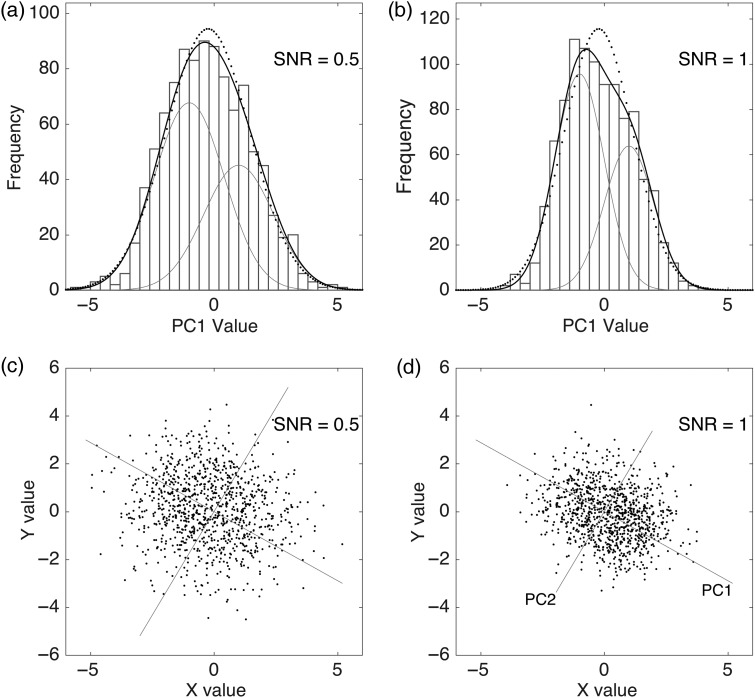
Illustrations of the identifiability problem in 1D and 2D. (a) Although a set of values comes from two populations of random numbers, the resulting distribution is essentially indistinguishable from a one-population distribution (dotted curve). (b) When the noise is variance is halved (SNR is increased), the two populations become distinguishable in the histogram. (c) Two populations in a two-dimensional space, also not distinguishable. (d) With twice the SNR, the principal component PC1 becomes visible, along which the two populations are separated. It is the projection of the values along PC1 that are depicted in (b).

References

-
- Clarke A C. (1973) Profiles of the Future: An Inquiry into the Limits of the Possible, p. 21 (Harper and Row, New York).
- Elmlund D, Elmlund H (2015) Cryogenic electron microscopy and single-particle analysis. Annu. Rev. Biochem. 84: 499–517. - PubMed
Publication types
MeSH terms
Substances
Grants and funding
LinkOut - more resources
Full Text Sources
Other Literature Sources