SLOPE-ADAPTIVE VARIABLE SELECTION VIA CONVEX OPTIMIZATION

Abstract

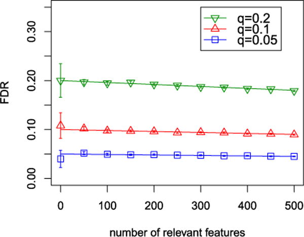
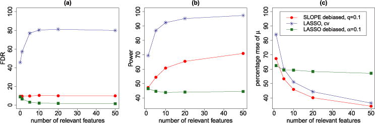
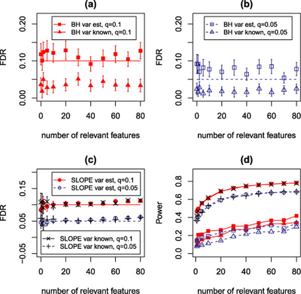
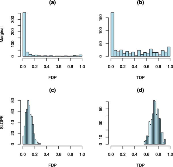
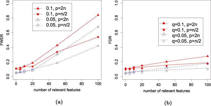
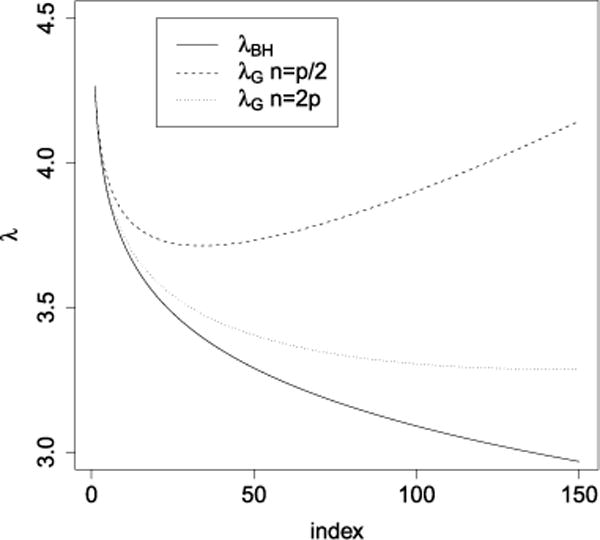
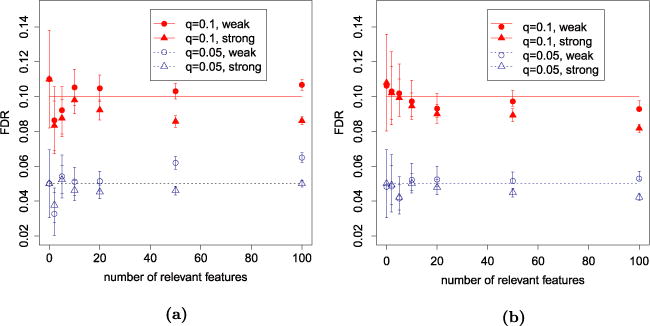
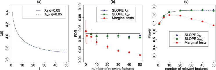
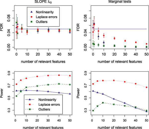
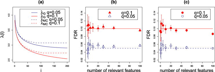
We introduce a new estimator for the vector of coefficients β in the linear model y = Xβ + z, where X has dimensions n × p with p possibly larger than n. SLOPE, short for Sorted L-One Penalized Estimation, is the solution to [Formula: see text]where λ₁ ≥ λ₂ ≥ … ≥ λ _p ≥ 0 and [Formula: see text] are the decreasing absolute values of the entries of b. This is a convex program and we demonstrate a solution algorithm whose computational complexity is roughly comparable to that of classical ℓ₁ procedures such as the Lasso. Here, the regularizer is a sorted ℓ₁ norm, which penalizes the regression coefficients according to their rank: the higher the rank-that is, stronger the signal-the larger the penalty. This is similar to the Benjamini and Hochberg [J. Roy. Statist. Soc. Ser. B57 (1995) 289-300] procedure (BH) which compares more significant p-values with more stringent thresholds. One notable choice of the sequence {λ _i } is given by the BH critical values [Formula: see text], where q ∈ (0, 1) and z(α) is the quantile of a standard normal distribution. SLOPE aims to provide finite sample guarantees on the selected model; of special interest is the false discovery rate (FDR), defined as the expected proportion of irrelevant regressors among all selected predictors. Under orthogonal designs, SLOPE with λ_BH provably controls FDR at level q. Moreover, it also appears to have appreciable inferential properties under more general designs X while having substantial power, as demonstrated in a series of experiments running on both simulated and real data.

Keywords: Lasso; Sparse regression; false discovery rate; sorted ℓ1 penalized estimation (SLOPE); variable selection.

FIG. 1

FDR of (1.5) in an orthogonal setting in which n = p = 5000. Straight lines correspond to q · p₀/p, marked points indicate the average False Discovery Proportion (FDP) across 500 replicates, and bars correspond to ±2 SE.

FIG. 2

Properties of different procedures as a function of the true number of nonzero regression coefficients: (a) FDR, (b) power, and (c) relative MSE defined as the average of $100\cdot {\Vert \widehat{\mu }-\mu \Vert }_{{\ell }_2}^2/{\Vert \mu \Vert }_{{\ell }_2}^2$ with μ = Xβ, $\widehat{\mu }=X\widehat{\beta }$. The design matrix entries are i.i.d. $\mathcal{N}\left(0,1/n\right),n=p=5000$, all nonzero regression coefficients are equal to $\sqrt{2\text{log}p}\approx 4.13,\text{and}{\sigma }^2=1$. Each point in the figures corresponds to the average of 500 replicates.

FIG. 3

Simulation results for testing multiple means from correlated statistics. (a)–(b) Mean FDP ± 2 SE for marginal tests as a function of k. (c) Mean FDP ± 2 SE for SLOPE. (d) Power plot.

FIG. 4

Testing example with q = 0.1 and k = 50. The top row refers to marginal tests, and the bottom row to SLOPE. Both procedures use the estimated variance components. Histograms of false discovery proportions are in the first column and of true positive proportions in the second.

FIG. 5

Observed (a) FWER for Lasso with λ_Bonf and (b) FDR for SLOPE with λ_BH under Gaussian design and n = 5000. The results are averaged over 500 replicates.

FIG. 6

Graphical representation of sequences {λ_i} for p = 5000 and q = 0.1. The solid line is λ_BH, the dashed (resp., dotted) line is λ_G given by (3.7) for n = p/2 (resp., n = 2p).

FIG. 7

Mean FDP ± 2 SE for SLOPE with ${\mathrm{\lambda }}_{{\mathrm{G}}^{\star }}$. Strong signals have nonzero regression coefficients set to $5\sqrt{2\text{log}p}$, while this value is set to $\sqrt{2\text{log}p}$ for weak signals. (a) p = 2n = 10,000. (b) p = n/2 = 2500.

FIG. 8

(a) Graphical representation of sequences λ_MC and λ_G for the SNP design matrix. (b) Mean FDP ± 2 SE for SLOPE with ${\mathrm{\lambda }}_{{\mathrm{G}}^{\star }}$ and λ_MC and for BH as applied to marginal tests. (c) Power of both versions of SLOPE and BH on marginal tests for ${\beta }_1=\cdots ={\beta }_k=1.2\sqrt{2\text{log}p}\approx 4.95,\sigma =1$. In each replicate, the signals are randomly placed over the columns of the design matrix, and the plotted data points are averages over 500 replicates.

FIG. 9

FDR and power of “scaled” SLOPE based on “gaussian” sequence ${\mathrm{\lambda }}_{{\mathrm{G}}^{\star }}$ (left panel) and BH-corrected single marker tests (right panel) for different deviations from the assumed regression model. Error bars for FDR correspond to mean FDP ± 2 SE.

FIG. 10

(a) Graphical representation of sequences λ_MC and λ_G for the variants design matrix. Mean FDP ± 2 SE for SLOPE with (b) ${\mathrm{\lambda }}_{{\mathrm{G}}^{\star }}$ and (c) λ_MC and for the variants design matrix and ${\beta }_1=\cdots ={\beta }_k=\sqrt{2\text{log}p}\approx 3.65,\sigma =1$.

FIG. 11

Estimated effects on HDL for variants in 17 regions. Each panel corresponds to a region and is identified by the name of a gene in the region, following the convention in Service et al. (2014). Regions with (without) previously reported association to HDL are on the green (red) background. On the x-axis variants position in base-pairs along their respective chromosomes. On the y-axis estimated effect according to different methodologies. With the exception of marginal tests—which we use to convey information on the number of variables and indicated with light gray squares—we report only the value of nonzero coefficients. The rest of the plotting symbols and color convention is as follows: dark gray bullet—BH on p-values from full model; magenta cross—forward BIC; purple cross—backward BIC; red triangle—Lasso–λ_Bonf; orange triangle—Lasso–λ_CV; cyan star—SLOPE– ${\mathrm{\lambda }}_{{\mathrm{G}}^{\star }}$; black circle—SLOPE with λ defined with Monte Carlo strategy.

FIG. 12

Each row corresponds to a variant in the set differently selected by the compared procedures, indicated by columns. Orange is used to represent rare variants and blue common ones. Squares indicate synonymous (or noncoding variants) and circles nonsynonimous ones. Variants are ordered according to the frequency with which they are selected. Variants with names in green are mentioned in Service et al. (2014) as to have an effect on LDL, while variants with names in red are not [if a variant was not in dbSNP build 137, we named it by indicating chromosome and position, following the convention in Service et al. (2014)].

References

1. Abramovich F, Benjamini Y. Wavelets and Statistics Lecture Notes in Statistics. Vol. 103. Springer; Berlin: 1995. Thresholding of wavelet coefficients as multiple hypotheses testing procedure; pp. 5–14.
1. Abramovich F, Benjamini Y, Donoho DL, Johnstone IM. Adapting to unknown sparsity by controlling the false discovery rate. Ann Statist. 2006;34:584–653. MR2281879.
1. Akaike H. A new look at the statistical model identification. (System identification and time-series analysis).IEEE Trans Automat Control. 1974;AC-19:716–723. MR0423716.
1. Barlow RE, Bartholomew DJ, Bremner JM, Brunk HD. Statistical Inference Under Order Restrictions The Theory and Application of Isotonic Regression. Wiley; New York: 1972. MR0326887.
1. Bauer P, Pötscher BM, Hackl P. Model selection by multiple test procedures. Statistics. 1988;19:39–44. MR0921623.
LinkOut - more resources