Where's the Noise? Key Features of Spontaneous Activity and Neural Variability Arise through Learning in a Deterministic Network

Abstract

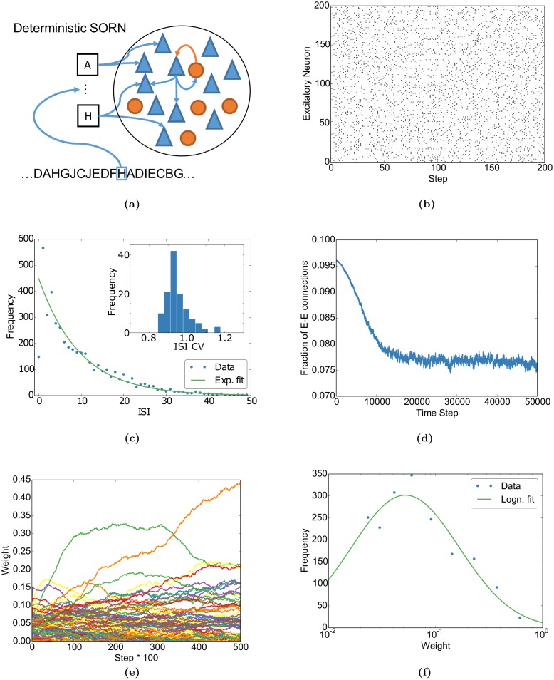
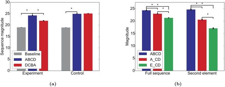
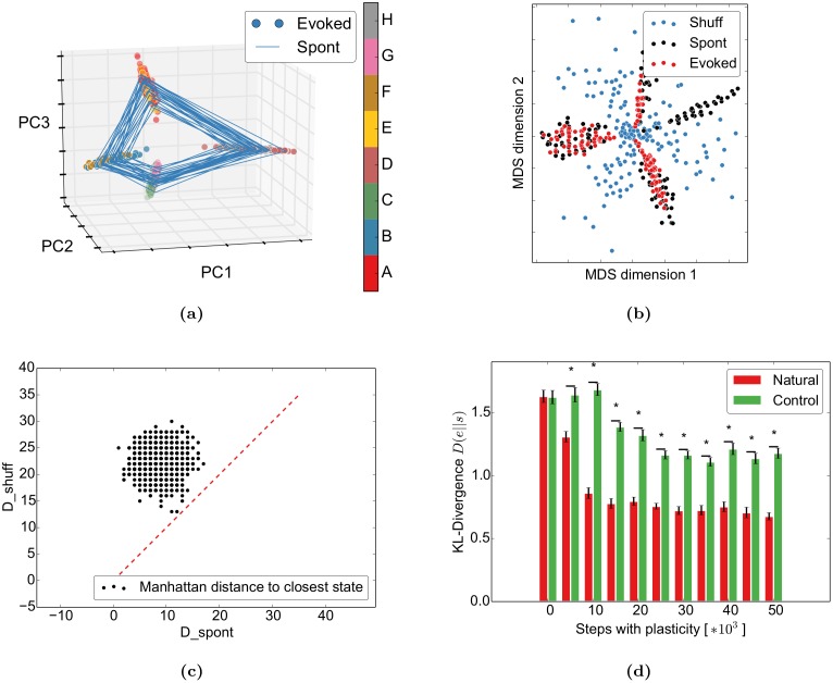
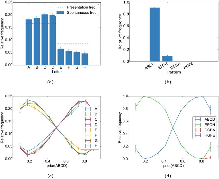
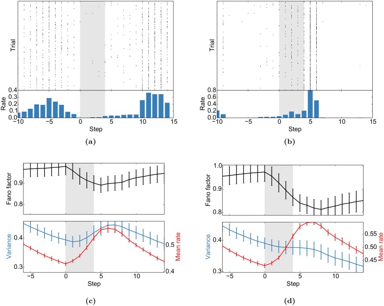
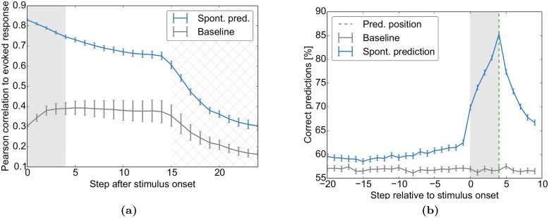
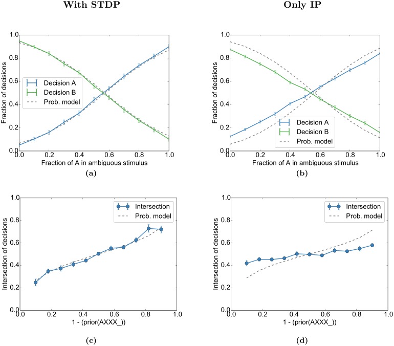
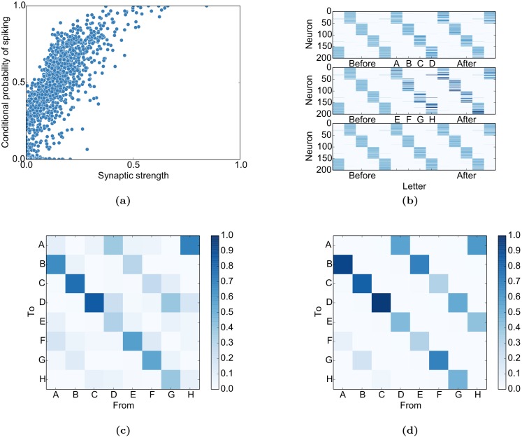
Even in the absence of sensory stimulation the brain is spontaneously active. This background "noise" seems to be the dominant cause of the notoriously high trial-to-trial variability of neural recordings. Recent experimental observations have extended our knowledge of trial-to-trial variability and spontaneous activity in several directions: 1. Trial-to-trial variability systematically decreases following the onset of a sensory stimulus or the start of a motor act. 2. Spontaneous activity states in sensory cortex outline the region of evoked sensory responses. 3. Across development, spontaneous activity aligns itself with typical evoked activity patterns. 4. The spontaneous brain activity prior to the presentation of an ambiguous stimulus predicts how the stimulus will be interpreted. At present it is unclear how these observations relate to each other and how they arise in cortical circuits. Here we demonstrate that all of these phenomena can be accounted for by a deterministic self-organizing recurrent neural network model (SORN), which learns a predictive model of its sensory environment. The SORN comprises recurrently coupled populations of excitatory and inhibitory threshold units and learns via a combination of spike-timing dependent plasticity (STDP) and homeostatic plasticity mechanisms. Similar to balanced network architectures, units in the network show irregular activity and variable responses to inputs. Additionally, however, the SORN exhibits sequence learning abilities matching recent findings from visual cortex and the network's spontaneous activity reproduces the experimental findings mentioned above. Intriguingly, the network's behaviour is reminiscent of sampling-based probabilistic inference, suggesting that correlates of sampling-based inference can develop from the interaction of STDP and homeostasis in deterministic networks. We conclude that key observations on spontaneous brain activity and the variability of neural responses can be accounted for by a simple deterministic recurrent neural network which learns a predictive model of its sensory environment via a combination of generic neural plasticity mechanisms.

Fig 1. Basic properties of the network match experimental findings.

(a) The Self-Organizing Recurrent Neural Network (SORN) consists of recurrently connected excitatory (blue) and inhibitory (red) deterministic McCulloch & Pitts threshold neurons. Each input letter (black boxes) stimulates an excitatory subpopulation. The excitatory recurrent connections are shaped by spike-timing dependent plasticity and synaptic normalization. The excitatory thresholds are regulated by intrinsic plasticity (see Methods for details). (b) Raster plot of spontaneous activity (no external input) after stimulating the network with ten randomly alternating letters during plasticity. (c) The inter-spike-interval (ISI) distribution of a randomly selected neuron during spontaneous activity is well-fitted by an exponential apart from very small ISIs. (c, inset) The distribution of coefficients of variation (CVs) of the ISIs clusters around one, as expected for exponential ISI distributions, compatible with the experimentally observed Poisson-like spiking [10, 40]. (d) The fraction of excitatory-to-excitatory connections converges to a stable fraction. (e) Individual weights fluctuate despite the global convergence as observed experimentally [41]. (f) After self-organization, i.e. at the end of (d), the binned distribution of excitatory-to-excitatory synaptic weights (dots) is well fit by a lognormal distribution (solid line, cp., e.g., [42]).

Fig 2. The network learns a predictive model mimicking [31].

Similar to [31], we stimulated the network either with the sequence “ABCD” (experiment) or with all permutations of this sequence (control). After a period of self-organization, the network was tested with the sequences “ABCD” and “DCBA”. (a) Mean firing rates (“sequence magnitude”) for both test sequences. (b) For the experimental condition, the network was also tested with the sequences “ABCD”, “A_CD”, and “E_CD”. Error bars represent SEM over 20 independent realizations. ⋆ indicates p < 0.05 for a two-sided t-test assuming independent samples and identical variances.

Fig 3. Spontaneous and evoked activity align through self-organization.

The network was stimulated with the words “ABCD” (67%) and “EFGH” (33%). (a) The spontaneous activity follows the spatiotemporal trajectories of the evoked states in the PCA projection. (b) In the multidimensional scaling projection, the evoked activity (red) follows the spontaneous outline (black) and avoids the shuffled spontaneous states (blue) (cp. Fig 6c of [13]). (c) The evoked states are closer to the spontaneous states than to the shuffled spontaneous states: As in Fig 6 of [13], the distance from evoked states to the closest spontaneous states (D_spont) is smaller than the distance to the closest shuffled spontaneous state (D_shuff). The red dashed line shows equality. (d) Spontaneous activity becomes more similar to evoked activity during learning: After self-organizing to “ABCD” and “EFGH” with identical probabilities, spontaneous activity was compared to the evoked activity from the imprinted sequences (natural) or the two control sequences “EDCBA” and “FGH” (control) with Kullback-Leibler divergence. New networks were generated for each training time and condition. Error bars represent SEM over 50 independent realizations. ⋆ indicates p < 0.05 for a t-test assuming independent samples and identical variances.

Fig 4. Different priors are learnt by the network.

During self-organization, the sequences “ABCD” and “EFGH” were randomly interleaved with frequencies of 67% and 33%, respectively. This is reflected in the relative occurrence of (a) each letter and (b) each word in the spontaneous activity. For different priors during self-organization, this results in the frequencies in (c) for each letter and in (d) for each word. Both show overlearning effects in that their frequencies are biased in favour of the word that was shown more often. The reversing trend and high variance for the extreme priors (0.1 and 0.9) can be accounted for by pathological network dynamics for some simulations with these priors. The letter frequency is the observed frequency in the evoked activity while the word frequency was normalized over the total number of observed words (“ABCD”, “EFGH”, “DCBA”, and “HGFE”) to yield better comparison over different realizations. Error bars represent SEM over 20 independent realizations.

Fig 5. Stimulus onset quenches variability.

(a) and (b) Sample spike trains from two representative neurons aligned to the stimulus presentation (shaded area). (c) and (d) The population average of the Fano factor (FF) decreases with stimulus onset. The FF is only computed for units that do not receive direct sensory input. These results mimic Fig 5 of [10]. FFs, mean rates and variances are for causal moving windows of 5 time steps. (c) was computed for the presentation of stimulus “AXXX_ _ _ …” during the test phase after being presented with a probability of 0.1 during self-organization. (d) In turn, “BXXX_ _ _ …” had a probability of 0.9 in the same experiment. Error bars represent SEM over 20 independent realizations.

Fig 6. Spontaneous activity predicts evoked activity and decisions.

The network self-organizes during repeated presentations of the sequences “AXXX_ _ _ …” (33%) and “BXXX_ _ _ …” (67%) with blank intervals in between. In the test phase, an ambiguous mix of cue “A” and cue “B” is presented (“A/BXXX_ _ _ …”, shaded area) and the network decides at the first “_” with a linear classifier if either A or B was the start of the sequence. (a) Trial-to-trial variability of the evoked activity patterns during the test phase is well predicted from activity prior to stimulus onset. The figure shows the correlation between the variable evoked activity patterns at different time steps after stimulus onset and a linear prediction of these based on the stimulus and either the spontaneous activity state prior to stimulus onset (blue) or trial-shuffled spontaneous activity (baseline, grey). Similar to Fig 4 in [8], the decay of the correlation is exponential-like. The correlation drops further as new stimuli are presented (hatched area). Due to variable inter-trial-intervals, the hatched area covers the entire area were stimulation is possible. (b) The decisions of the network can be predicted from spontaneous activity before stimulus onset. The plot shows the accuracy of predicted network decisions (“A” vs. “B”) at the green dashed line from activity surrounding the decision. Separate classifiers were trained for each of the 11 ambiguity classes (e.g. 20%A) and time step surrounding the decision. The grey line corresponds to predictions from trial-shuffled activity. Predictions in (b) are averaged over all priors of Fig 7c. Error bars represent SEM over 20 independent realizations.

Fig 7. Prior and ambiguous information is combined in network decisions.

(a) As in Fig 6, the network self-organizes during repeated presentations of the sequences “AXXX_ _ _ …” (33%) and “BXXX_ _ _ …” (67%) with blank intervals in between. In the test phase, an ambiguous mix of cue “A” and cue “B” is presented (“A/BXXX_ _ _ …”) and the network decides at the first “_” with a linear classifier if either A or B was the start of the sequence. The fraction of decisions for “A” or “B” at the first blank state “_” approximates the integration of cue likelihood and prior stimulus probability as expected from the probabilistic model (grey dashed line) for the given prior (p(A) = 0.33). The probabilistic model was fitted by grid search over its two parameters to the parameters that had the smallest accumulated error over all priors. (b) For the “Only IP” condition, STDP was deactivated during the self-organization phase and a new probabilistic model was fitted. (c, d) The intersections of the decisions for different priors for our simulations (blue line) and the probabilistic model (grey dashed). The performance was evaluated for the same simulation as Figs 5 and 6. Error bars represent SEM over 20 independent realizations.

Fig 8. Self-organization imprints stimulus properties in the network.

(a) The conditional probability of x _i spiking given that x _j just spiked (p(x _i(t + 1) = 1|x _j(t) = 1)) is roughly proportional to their synaptic connection $W_{ij}^{EE}$ except for saturation effects for very large weights. (b) The firing probabilities of each neuron relative to stimulus onset. The network develops sequential activity patterns during the presentation of both sequences (top and middle) and during spontaneous activity (aligned to spontaneous states corresponding to “C”, bottom). Neurons were sorted according to their maximal firing probability relative to the sequence “ABCD”. (c) The prediction of transition probabilities during spontaneous activity from the singular value decomposition of W ^EE. (d) The actual transition probabilities during spontaneous activity show intermediate switching between the two sequences probably due to variability introduced by intrinsic plasticity (see Discussion for details).

References

1. Laughlin S, de Ruyter van Steveninck R, Anderson J. The metabolic cost of neural information. Nature Neuroscience. 1998;1(1):36–41. 10.1038/236 - DOI - PubMed
1. Faisal AA, Selen LPJ, Wolpert DM. Noise in the nervous system. Nature Reviews Neuroscience. 2008;9(4):292–303. 10.1038/nrn2258 - DOI - PMC - PubMed
1. Mainen ZF, Sejnowski TJ. Reliability of spike timing in neocortical neurons. Science. 1995;268(5216):1503–6. 10.1126/science.7770778 - DOI - PubMed
1. Schneidman E, Freedman B, Segev I. Ion channel stochasticity may be critical in determining the reliability and precision of spike timing. Neural Computation. 1998;10(7):1679–703. 10.1162/089976698300017089 - DOI - PubMed
1. Hardingham NR, Larkman AU. Rapid report: the reliability of excitatory synaptic transmission in slices of rat visual cortex in vitro is temperature dependent. The Journal of Physiology. 1998;507:249–56. 10.1111/j.1469-7793.1998.249bu.x - DOI - PMC - PubMed
Publication types
LinkOut - more resources