Wilson-Cowan Equations for Neocortical Dynamics

Abstract

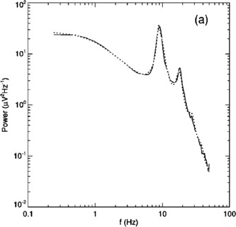
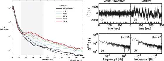
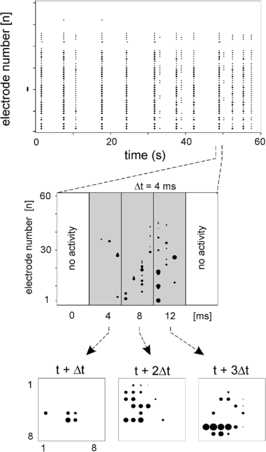
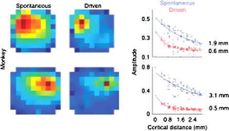
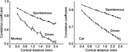
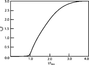
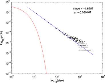
In 1972-1973 Wilson and Cowan introduced a mathematical model of the population dynamics of synaptically coupled excitatory and inhibitory neurons in the neocortex. The model dealt only with the mean numbers of activated and quiescent excitatory and inhibitory neurons, and said nothing about fluctuations and correlations of such activity. However, in 1997 Ohira and Cowan, and then in 2007-2009 Buice and Cowan introduced Markov models of such activity that included fluctuation and correlation effects. Here we show how both models can be used to provide a quantitative account of the population dynamics of neocortical activity.We first describe how the Markov models account for many recent measurements of the resting or spontaneous activity of the neocortex. In particular we show that the power spectrum of large-scale neocortical activity has a Brownian motion baseline, and that the statistical structure of the random bursts of spiking activity found near the resting state indicates that such a state can be represented as a percolation process on a random graph, called directed percolation.Other data indicate that resting cortex exhibits pair correlations between neighboring populations of cells, the amplitudes of which decay slowly with distance, whereas stimulated cortex exhibits pair correlations which decay rapidly with distance. Here we show how the Markov model can account for the behavior of the pair correlations.Finally we show how the 1972-1973 Wilson-Cowan equations can account for recent data which indicates that there are at least two distinct modes of cortical responses to stimuli. In mode 1 a low intensity stimulus triggers a wave that propagates at a velocity of about 0.3 m/s, with an amplitude that decays exponentially. In mode 2 a high intensity stimulus triggers a larger response that remains local and does not propagate to neighboring regions.

Keywords: Bogdanov–Takens bifurcation; Directed percolation phase transition; Localized decaying LFP and VSD responses; Neural network master equation; Pair-correlations; Propagating decaying LFP and VSD waves; Wilson–Cowan equations.

Fig. 1

The upper trace is the first recording of spontaneous electrical activity from the human scalp. The lower trace is a 10 Hz oscillation. [Reproduced from [3]]

Fig. 2

The power spectrum of the occipital EEG of a resting, awake human. [Reproduced from [4]]

Fig. 3

The left panel shows the function $75/(3+f^2)$, the right panel the fit of such a function to the EEG power spectrum shown in Fig. 2

Fig. 4

The left panel shows the power spectra of LFP recordings from a cat’s visual cortex in response to sine-wave modulated grating patterns. [Reproduced from [5].] The right panel shows fMRI recordings of both resting and stimulated human brain activity, and their associated power spectra. [Reproduced from [6]]

Fig. 5

Electrode data from slices of rat neocortex. The top graph is a raster plot of electrode activation times. They seem synchronous, but closer examination reveals that the times exhibit self-similarity. The bottom graphs show a sequence of electrode activations in the original array. [Reproduced from [9]]

Fig. 6

Probability distribution of burst sizes at different bin widths Δt. Inset: Dependence of slope exponent α on bin width. [Reproduced from [9]]

Fig. 7

Spikes of low amplitude initiate traveling waves of LFP in the cortex. See text for details. [Reproduced from [13]]

Fig. 8

Spikes of larger amplitude initiate standing waves of LFP in the cortex. See text for details. [Reproduced from [13]]

Fig. 9

Fall of with distance of cortical pair correlations. See text for details. [Reproduced from [13]]

Fig. 10

The left panel shows the E–I phase plane and nullclines of Eq. (7). The intersections of the two null clines are equilibrium or fixed points of the equations. Those labeled (+) are stable, those labeled (−) are unstable. Parameters: $w_{EE}=12$, $w_{EI}=4$, $w_{IE}=13$, $w_{II}=11$, $n_H=0$. The stable fixed points are nodes. The right panel shows an equilibrium which is periodic in time. Parameters: $w_{EE}=16$, $w_{EI}=12$, $w_{IE}=15$, $w_{II}=3$, $n_H=1.25$. In this case the equilibrium is a limit cycle. [Redrawn from [24]]

Fig. 11

The left panel shows bifurcations of Eq. (7) in the spatially homogeneous case, organized around the Bogdanov–Takens (BT) bifurcation. SN1 and SN2 are saddle-node bifurcations. AH is an Andronov–Hopf bifurcation, and SHO is a saddle homoclinic-orbit bifurcation. Note that a and b are the control parameters introduced earlier. The right panel shows the nullcline structure of a Bogdanov–Takens bifurcation. At the Bogdanov–Takens point, a stable node (open circle) coalesces with an unstable point. [Redrawn from [34]]

Fig. 12

Neural state transitions. a is the activated state of a neuron. q is the quiescent state. α is a decay constant, but f depends on the number of activated neurons connected to the neuron, and on an external stimulus h

Fig. 13

The firing rate function $f[s_E(n)]$, ${\tau }_m=1/\alpha =3\text{ms}$ is the neural membrane time constant, I is the input current, and $I_{\mathrm{RH}}$ is the rheobase or threshold current

Fig. 14

Raster plot of the spiking patterns in a network of $N=800$ excitatory neurons. Each black dot represents a neural spike. The mean activity $\langle n_E(t)\rangle$ is represented by the blue trace. Simulation using the Gillespie algorithm with parameter values $h_E=h_I=0.001$, $w_0=w_E-w_I=0.2$, and $w_E+w_I=0.8$. [Redrawn from [35]]

Fig. 15

Phase plane plots of the activity shown in Fig. 14 showing the vector field (blue) and nullclines $\dot{E}=0$ (magenta) and $\dot{I}=0$ (red), of Eq. (1) and plots of a deterministic (black) and a stochastic (green) trajectory starting from identical initial conditions. [Redrawn from [35]]

Fig. 16

Raster plot of the spiking patterns in a network of $N=800$ excitatory neurons. Each black dot represents a neural spike. The mean activity $\langle n_E(t)\rangle$ is represented by the blue trace. Simulation using the Gillespie algorithm with parameter values $h_E=h_I=0.001$, $w_0=w_E-w_I=0.2$, and $w_E+w_I=13.8$. [Redrawn from [35]]

Fig. 17

Phase plane plots of the activity shown in Fig. 16 showing the vector field (blue) and nullclines $\dot{E}=0$ (magenta) and $\dot{I}=0$ (red), of Eq. (1) and plots of a deterministic (black) and a stochastic (green) trajectory starting from identical initial conditions. [Redrawn from [35]]

Fig. 18

Network burst distribution in number of spikes, together with geometric (red) and power law (blue) fit; Δt, the mean inter-spike interval, is the time bin used to calculate the distribution, and $\beta =-1.62$ is the slope exponent of the fit. Simulation using the Gillespie algorithm with parameter values $h_E=h_I=0.001$, $w_0=w_E-w_I=0.2$, and $w_E+w_I=0.8$. [Redrawn from [35]]

Fig. 19

Network burst distribution in number of spikes, together with geometric (red) and power law (blue) fit; Δt, the mean inter-spike interval, is the time bin used to calculate the distribution, and β is the slope exponent of the fit. Simulation using the Gillespie algorithm with parameter values $h_E=h_I=0.001$, $w_0=w_E-w_I=0.2$, and $w_E+w_I=13.8$. [Redrawn from [35]]

Fig. 20

The left panel shows the pair-correlation function for resting and driven activity, for additive Gaussian noise, the right panel that for resting and driven activity, for intrinsic noise, averaged over many simulations using the Gillespie algorithm. [Reproduced from [38]]

Fig. 21

A Variation in the LFP amplitude of decaying waves. The largest amplitude is the initial response to a brief weak current pulse. B The exponential decay of the LFP amplitude, as a function of distance traveled. C Time–distance plot of the peak amplitude indicating that the velocity of wave propagation is constant at about $0.3\text{m}{\text{s}}^{-1}$. D Localized LFP in response to a strong current pulse. E Rapid decay of the amplitude in a linear fashion. F Very slow propagation of the LFP

References

1. Sholl DA. The organization of the cerebral cortex. London: Methuen; 1956.
1. Caton R. Br Med J. 1875;2:278.
1. Berger H. Arch Psychiatr Nervenkrankh. 1929;87:527–570. doi: 10.1007/BF01797193. - DOI
1. Rowe DL, Robinson PA, Rennie CJ. J Theor Biol. 2004;231:413–433. doi: 10.1016/j.jtbi.2004.07.004. - DOI - PubMed
1. Henrie JA, Shapley R. J Neurophysiol. 2005;94:479–490. doi: 10.1152/jn.00919.2004. - DOI - PubMed
LinkOut - more resources