The functional diversity of retinal ganglion cells in the mouse

Abstract

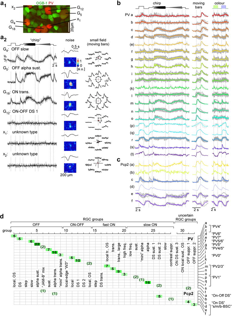
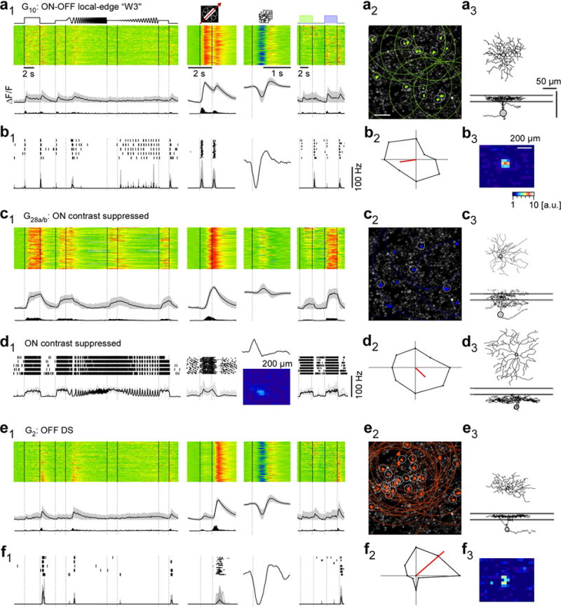
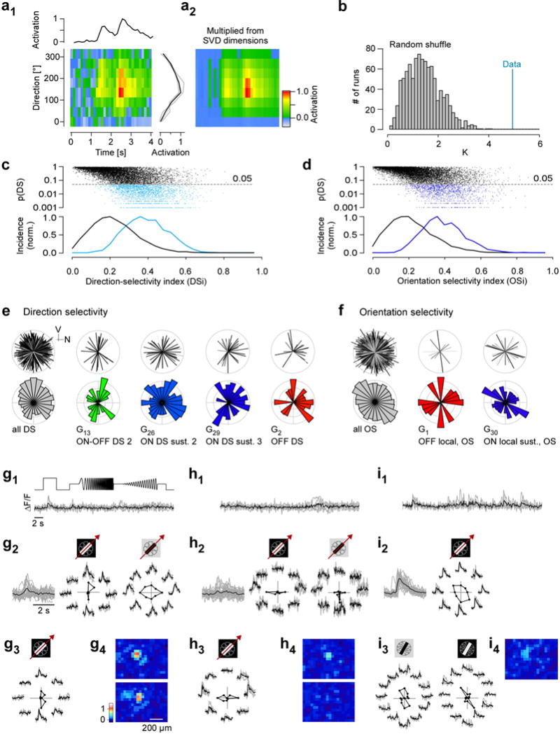
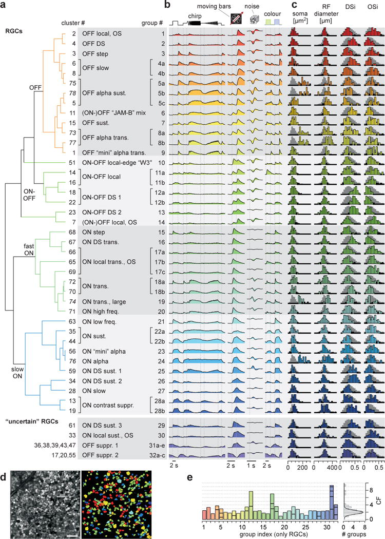
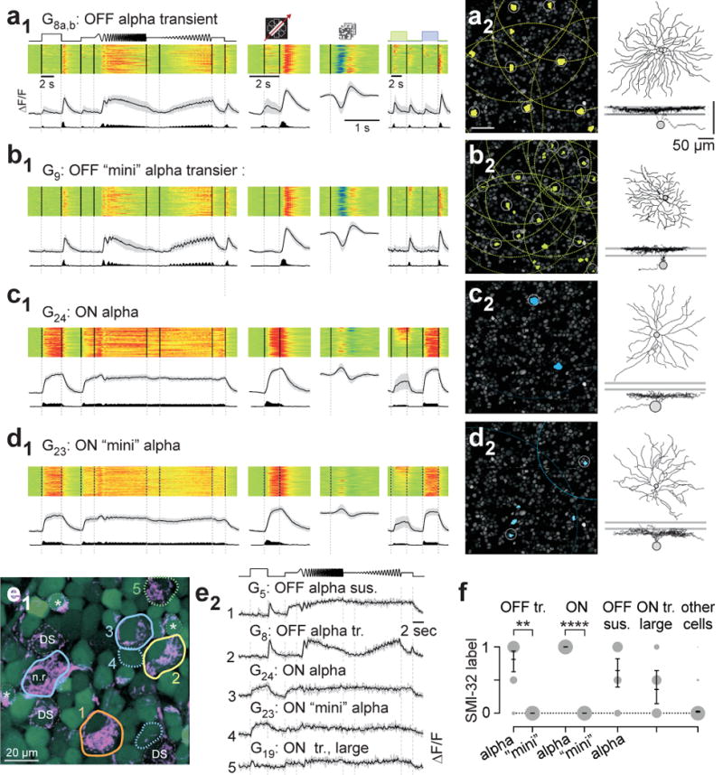
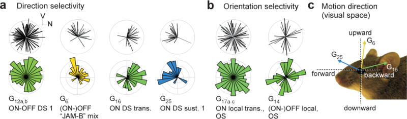
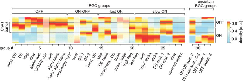
In the vertebrate visual system, all output of the retina is carried by retinal ganglion cells. Each type encodes distinct visual features in parallel for transmission to the brain. How many such 'output channels' exist and what each encodes are areas of intense debate. In the mouse, anatomical estimates range from 15 to 20 channels, and only a handful are functionally understood. By combining two-photon calcium imaging to obtain dense retinal recordings and unsupervised clustering of the resulting sample of more than 11,000 cells, here we show that the mouse retina harbours substantially more than 30 functional output channels. These include all known and several new ganglion cell types, as verified by genetic and anatomical criteria. Therefore, information channels from the mouse eye to the mouse brain are considerably more diverse than shown thus far by anatomical studies, suggesting an encoding strategy resembling that used in state-of-the-art artificial vision systems.

Figure E1. Linking electrophysiology and imaging data (related to Fig. 1)

a, simultaneously recorded RGC Ca²⁺ (top) and spiking (bottom) activity in response to binary spatial dense noise stimulation. b, average Ca²⁺ event triggered by a single spike, averaged across n=6 cells (shading = 1 s.d.); event decay was fit (red) using a single exponential (for time constant τ, see inset, mean ± 1 s.d.) to yield an estimated impulse response. A linear prediction of Ca²⁺ (calculated by convolution of the impulse response with binarised spike-traces) was compared to measured values to estimate the mean nonlinearity (c). d, Ca²⁺ (top) and spiking (bottom) response to the full-field “chirp” stimulus (Methods) simultaneously recorded in an RGC (red trace, Ca²⁺ signal predicted from spiking response). e, number of scan fields as a function of blue-green index (BGi, see Methods) averaged over all ROIs in each field (cf. Fig. 1a₁).

Figure E2. Clustering and grouping (related to Fig. 2)

a–c. Selection of cluster size and cluster quality/consistency analysis. a, normalised Bayesian Information Criterion (BIC) curves for non-DS (black) and DS (blue) cells. Arrows indicate the optimal numbers of clusters. b, rank-ordered posterior probability curves indicating cluster quality. Curves were normalised for cluster size and averaged for non-DS (black) and DS (blue) clusters separately. Shaded area indicates 1 s.d. across clusters. c, histogram of median correlation between the original clusters and clusters identified on 20 surrogate datasets, created by repeated subsampling of 90% of the original dataset (bootstrapping); for each cluster, the best matching cluster from the original clustering was selected. d, heat maps of Ca²⁺ responses (d₁) to the 4 visual stimuli (cf. Fig. 1) of n=11,210 cells from 50 retinas. Shown are raw data sorted by the response to the colour stimulus. Each line represents responses of a single cell with activity colour-coded such that warmer colours represent increased activity. Temporal features (d₂) were extracted from the cells’ light responses (Methods) and used for automatic clustering (d₁ → e₁). e, heat maps showing clustered data (e₁, n=72 clusters plus cells discarded based on signal-to-noise (S/N) ratio), with block height representing the number of included cells. Distributions of S/N (e₂, top) and GAD67 labelling (e₂, bottom) used to discard clusters and sort the remaining ones into retinal ganglion cells (RGCs), “uncertain” RGCs and displaced amacrine cells (dACs). f, heat maps showing n=46 groups (divided into n=32 RGC groups, including n=4 “uncertain” ones, and n=14 dAC groups; sorted by response similarities) after re-clustering of large-soma cells (alpha cell post-processing, see panels g,h). g, distribution of region of interest (ROI) area (as proxy for soma size) for all cells classified as RGCs and “uncertain” (e₂). Inset: same distribution but on a log-scale. Dashed line marks threshold to separating large-soma cells (Methods). h, results of re-clustering of large-soma cells (from g): heat maps show light-evoked Ca²⁺ responses to the 4 visual stimuli (cf. Fig. 1b). Clusters that resulted in new RGC groups are indicated; the remaining cells stayed with their original clusters.

Figure E3. Group overview – Functional groups classified as “uncertain” RGCs and displaced amacrine cell (dAC) in the mouse retina (related to Fig. 2)

a, clusters organised according to hierarchical trees (dendrograms, see Methods) and grouped based on functional similarity (see main text for details), resulting in n=4 “uncertain” RGC (top) and n=14 dAC groups (bottom). b, mean Ca²⁺ responses to the 4 stimuli (cf. Fig. 1b) for each cluster. c, histograms of selected properties, from left to right: ROI (soma) area, receptive field (RF) diameter (2 s.d. from Gaussian fit; see Fig. 1b₁ and Fig. E4), DS and OS indices (DSi and OSi, respectively, Methods). For details on each cluster, see also SI Data 1_40–49 (“uncertain”), and SI Data 1_50–75 (dACs). d, example experiment (left, from Fig. 1a₂); centre: showing dACs (lilac) and “uncertain” RGCs (blue); right: colour-coded by broad categories, as in (e). e, total number of cells (top) and percentage of cells in sets of groups (bottom) per experiment (only experiments with ≥198 cells) illustrating consistency across experiments. Scale bar: d, 50 μm.

Figure E4. Relationship between RGC receptive field centres and their dendritic arbours (related to Fig. 2)

a, receptive field (RF) centre maps of a G₈ transient OFF alpha RGC (a₁) and a G₂ small-field RGC (a₂), with their reconstructed morphologies overlaid. 1- and 2-s.d. contours of RF centres fitted with 2D Gaussians are indicated by blue and red ovals, respectively. b, area of RF centre fits from (a) as function of dendritic arbour area (n=18 RGCs). Scale bar: 100 μm.

Figure E5. Mapping RGC groups onto genetic types – Functional diversity of PV- and Pcp2-positive RGCs (related to Fig. 2)

a, diversity of PV-positive RGCs (red) in a PV:tdTomato mouse retina electroporated with OGB-1 (a₁, green). Ca²⁺ responses and receptive fields (a₂) from 6 PV-positive cells in exemplary field are shown (black, mean response, grey, single trials). The top four cells could be clearly matched to RGC groups (cf. Fig. 2), whereas the remaining two (x₁, x₂) were discarded due to the lack of responses to both full-field and moving bar stimuli; note, however that both cells yielded a clear RF. b, Ca²⁺ responses of functionally distinct PV-RGC groups (20 response types PV a-t, thereof 14 with n ≥ 3 cells). Traces colour-coded by group assignment (colours as in Fig. 2) represent mean responses, with individual cell responses in grey. c, same for Pcp2-positive (6 response types Pcp2 a-f, thereof 3 with n ≥ 3 cells) RGC groups. d, table illustrating the relationship between RGC groups (Fig. 2) and functional PV- and Pcp2-positive RGC types from (a,b). Numbers represent the total cell count of each allocation. Names in quotes (e.g. “PV5”) refer to the cells’ original names (see PV- and Pcp2-study).

Figure E6. Examples of RGC groups

a, functional “fingerprint” of G₁₀ RGCs, identified as local-edge-detector (W3) cells. Light-evoked Ca²⁺ responses of n=149 cells (a₁): heat maps (top) illustrating individual responses, with response averages and firing rates estimated from Ca²⁺ signals (cf. Fig. E1a–d) below. Ganglion cell layer (a₂; experiment from Fig. 1a₂) with G₁₀ somata (green) and receptive fields (RFs, dotted) indicated. Grey circles mark cells with RFs that passed a quality criterion (Methods). Example morphology of a G₁₀ cell filled after electrical single-cell recording (a₃, cf. b). For a complete summary of the group’s properties, see SI Data 2₁₀. b, electrical single-cell recording of a G₁₀ cell: spiking responses as raster plots and mean spike rates for “chirp”, moving bar and blue/green stimuli as well as time kernel derived from noise stimulus (b₁), polar plot of responses to moving bar (b₂) and RF map (b₃) c_1,2, G_28a,b (n=100) contrast-suppressed ON RGCs with sample morphology (c₃; G_28a,b cell dye-injected after Ca²⁺ imaging). d_1,2, electrical single-cell recording of a contrast-suppressed ON RGC with different morphology (d₃ vs. c₃). e,f, G₂ direction-selective OFF RGCs (n=162) that stratify between the ChAT bands (e₃), as fingerprint (e_1,2) and exemplary electrical single-cell recording (f_1–3). Scale bars: 50 μm; grey lines in a₃,c₃,d₃,e₃: ChAT bands.

Figure E7. Direction and orientation selectivity (related to Fig. 4)

a, (a₁) stimulus direction vs. time map for an exemplary direction selective RGC with temporal (top) and directional (right) activation profiles shown; Singular Value Decomposition (SVD) was used to estimate the time-course and tuning function; individual stimulus repeats in grey, average in black. (a₂) Reconstruction of direction vs. time map based on time course and tuning function of extracted by SVD. b, statistical significance testing for direction selectivity (DS) or orientation selectivity (OS) was performed by projecting the direction/orientation profile on a single (for DS) or double (for OS) period cosine (blue) and the magnitude of the projection to the distribution of projections obtained by randomly permuting tuning-angles from the original data (grey; bootstrapping). The p-value is obtained by computing the percentile of the data (blue) in the bootstrap distribution (grey). c, d, p-values for direction (c) and orientation (d) tuning as function of the respective selectivity index (top, scatter plot; bottom, histogram; black, non-DS cells; light blue, DS cells; dark blue, OS cells). Note that tuning probability (p_DS, p_OS) only partially predicted tuning strength (DSi, OSi). e, pairs of polar plots showing the distribution of preferred motion directions for all direction-selective (DS) RGCs together and for all DS RGC groups not shown in Fig. 4, (V, ventral; N, nasal direction; same group colour code as in Fig. 2). Top plot of each pair: the cells’ individual preferred directions, with line length representing DSi and line grey level p(DS) (Methods). Bottom plot of each pair: circular histogram of preferred direction. f, like (a) but for orientation-selective (OS) RGCs. g–i, exemplary OS RGCs, illustrating the functional diversity within G₁₇ (local ON trans. OS cells); none of them display strong full-field responses (g₁,h₁,i₁, left). A “vertically-tuned” ON OS cell (g₂, left) that shows little tuning to a dark moving bar (g₂, right; g₃, another example). Note the lobular structures bracketing the RF centre (coloured RF maps in g₄). Two examples for “horizontally-tuned” ON OS cells (h_2,3) with their respective RF maps (h₄). ON OS cell that shows weak tuning to bright moving bars (i₁, left) but strong OS to stationary bright and dark bars (i_2–4, centre and right, respectively; Methods).

Figure E8. Retinal distribution of PV-positive cells in the PV^Cre × Ai9^tdTomato mouse line (related to Fig. 2)

a,b, density map (a) and magnified sample areas (b) illustrate PV-labelling anisotropy.

Figure E9. Mapping RGC groups to morphologies

a–c, exemplary morphologies of RGCs filled after electrical recording or Ca²⁺ imaging and subsequently clustered/sorted into specific RGC groups or discarded (c, right) based on their light response S/N. Scale bars: 50 μm.

Figure E10. RGC groups cover a basic feature space

a,b, relationship of four basic response indices of RGC groups. Disc-area shows group size. Indices capture preference for stimulus polarity (ON-OFF index; Methods), for high vs. low temporal frequencies and contrasts (see below), as well as the full-field index (FFi; Methods), which reflects response preference for global (full-field “chirp”) versus local (moving-bar) stimulation. Contrast- and Frequency-indices represent contrasts of feature activation ( $\left(F_j-F_k\right)/\left(F_j+F_k\right)$) at respective time points during the full-field “chirp” stimulus, with j=12, k=9 for frequency, and j=17, k=15 for contrast. Before calculating ratios, feature activation (F) was normalised (0…1) by passing values through a cumulative normal distribution.

Figure 1. Data collection

a, whole-mounted mouse retina, electroporated with OGB-1 and recorded with a two-photon microscope (64×64 pixel @ 7.8 Hz) in the GCL. Scan fields (a₁, left; 110×110 μm) comprised 80 ± 20 cells. Regions-of-interest (ROIs) (a₁, right), were placed semi-automatically. Montage (a₂) of 9 consecutively recorded fields (rectangles; a₁ in red). b, Ca²⁺ signals from 7 ROIs colour-coded in (a₁). Single trials in grey, averages of n=4 (“chirp”, green/blue) or 24 (moving bars) trials in black (b₁). Responses to 4 visual stimuli (b₁): Full-field “chirp”, bright bars moving in 8 directions, full-field alternating green/blue and binary noise for space-time kernels. Direction- and orientation-selectivity (b₂): Traces by motion direction; polar plot of peak response, vector sum in red. c, left: experiment in (a) immunostained for GAD67 (green; GABAergic ACs) and ChAT (red; starburst-ACs). Right: from (a₁); both images show same colour-coded ROIs (left, dots, right, ROI outlines) and starburst-ACs (white dots): cell 6 is GAD67-positive, cell 7 is a starburst-AC. d, OGB-1 (green) electroporated retina from transgenic mice with tdTomato (red) expressed in sets of RGCs (top: PV; bottom: Pcp2). e, simultaneous Ca²⁺ imaging and electrical recording: dye-filled, anatomically reconstructed cell (e₁, top: whole-mount; bottom: profile, lines mark ChAT bands). Light responses (e₂) from top to bottom: spike raster and rate (20 ms bins), recorded (black) and reconstructed (orange) Ca²⁺ signal. Scale bars: 50 μm unless indicated.

Figure 2. Functional RGC types of the mouse retina

a, cluster-dendrogram (Methods) with groups indicated: n=28 RGC and n=4 “uncertain” RGC groups. b, cluster-mean Ca²⁺ responses to the 4 stimuli. c, selected metrics, from left to right: ROI (soma) area, receptive field (RF) diameter (2 s.d. of Gaussian), DS-index and OS-index (Methods). Background-histograms demarcate all RGCs. d, experiment (left, from Fig. 1a₂) with RGCs colour-coded by group (right). dACs and discarded cells not shown. e, Coverage factor (CF) calculated from RF-area for RGC groups, with horizontal divisions delineating individual clusters (left) and distribution of CFs across groups (right). Scale bar in d, 50 μm.

Figure 3. Classical alpha RGCs and their “mini” counterparts

a, functional “fingerprint” of classical transient OFF alpha cells (G_8a,b). Light-evoked Ca²⁺ responses of n=80 cells (a₁): heat-maps (top) of individual responses, response averages and firing rates estimated from Ca²⁺ signals below (cf. Extended Data Fig. E1). a₂, left, G_8a,b somata (yellow) and receptive fields (RFs, dotted) indicated in example experiment (cf. Fig. 1a₂). Grey circles mark cells with RFs above quality criterion (Methods). Sample morphology of a G_8a,b cell filled after electrical single-cell recording (a₂, right). For details, see SI Data 2₈. b_1,2, G₉ RGCs (n=68), dubbed transient OFF mini alpha because of their similarity in light response to G_8a,b RGCs (cf. a_1,2). c_1,2, G₂₄ RGCs (n=44), identified as classical ON alpha. d_1,2, G₂₃ RGCs (n=113), dubbed ON mini alpha (cf. c_1,2). Mini alphas have smaller RF diameters than classical alphas (median in μm, 95% confidence interval): G₉,280 (270–293) versus G₈, 306 (294–315) with p=0.01232), and G₂₃, 236 (218–256) versus G₂₄, 319 (290–352) with p=0.00026 (rank-sum test). e, overlay of OGB-1-stained cells (green) and SMI-32 (magenta). SMI-32-positive RGCs include classical alphas (e₁, solid contours; n.r. indicates a non-responsive cell), one large-soma non-alpha cell (green, dotted contour) as well as weakly-labeled ON-OFF DS cells (dashed contours) and starburst-ACs (asterisks). Mini alpha cells (blue, dotted contours) are SMI-32-negative. Chirp-evoked Ca²⁺ responses (e₂) for 5 cells in (e₁). f, SMI-32 statistics (OFF tr.: alpha, n=16, mini, n=3; ON: alpha, n=6, mini, n=15; OFF sus. alpha, n=14; ON tr. large, n=7; other, n=957; means with 95% confidence intervals, **, p≤0.01; ****, p≤0.0001, logistic regression).

Figure 4. Direction- and orientation-selectivity

a, pairs of retinocentric polar plots showing distributions of preferred motion directions of selected direction-selective (DS) RGC groups (V, ventral; N, nasal). Top, plot of each pair: preferred directions, with length representing DSi and grey level p(DS) (Methods). Bottom, plot of each pair: circular area-normalised histogram. b, like (a), selected orientation-selective (OS) RGCs. Further DS/OS groups detailed in Extended Data Fig. E7. c, motion directions in the visual space of the mouse.

Figure 5. Mapping RGC groups to morphologies

Heat map of each RGC group’s estimated dendritic stratification across the IPL (cf. Fig. 2); ON/OFF sublaminae and ChAT bands indicated. Warmer colours represent higher dendritic densities (Methods). Shaded IPL profiles indicate deviation from known stratification pattern (G₆) or an unexpected pattern given a potentially novel group’s response polarity (G_11,18,19).

References

1. Masland RH. The neuronal organization of the retina. Neuron. 2012;76:266–280. - PMC - PubMed
1. Euler T, Haverkamp S, Schubert T, Baden T. Retinal bipolar cells: elementary building blocks of vision. Nat Rev Neurosci. 2014;15:507–19. - PubMed
1. Lettvin J, Maturana H, McCulloch W, Pitts W. What the Frog’s Eye Tells the Frog’s Brain. Proc IRE. 1959;47:1940–1951.
1. Werblin FS, Dowling JE. Organization of the retina of the mudpuppy, Necturus maculosus. II Intracellular recording. J Neurophysiol. 1969;32:339–355. - PubMed
1. Cleland BG, Levick WR. Brisk and sluggish concentrically organized ganglion cells in the cat’s retina. J Physiol. 1974;240:421–456. - PMC - PubMed
Publication types