Automated Reconstruction of Three-Dimensional Fish Motion, Forces, and Torques

Abstract

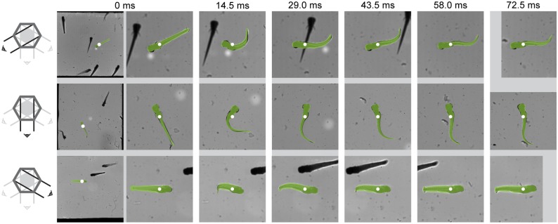
Fish can move freely through the water column and make complex three-dimensional motions to explore their environment, escape or feed. Nevertheless, the majority of swimming studies is currently limited to two-dimensional analyses. Accurate experimental quantification of changes in body shape, position and orientation (swimming kinematics) in three dimensions is therefore essential to advance biomechanical research of fish swimming. Here, we present a validated method that automatically tracks a swimming fish in three dimensions from multi-camera high-speed video. We use an optimisation procedure to fit a parameterised, morphology-based fish model to each set of video images. This results in a time sequence of position, orientation and body curvature. We post-process this data to derive additional kinematic parameters (e.g. velocities, accelerations) and propose an inverse-dynamics method to compute the resultant forces and torques during swimming. The presented method for quantifying 3D fish motion paves the way for future analyses of swimming biomechanics.

Fig 1. Schematic overview of the tracking method.

We provide initial information by creating a 3D model of the fish, calibrating the cameras and initialising the fish position by clicking the snout and tail position in the images from every camera (I). For every time step, we segment the fish in the images from all cameras and predict the fish position, orientation and body curvature based on previous frames (II). The predicted parameters are then used to initialise an optimisation algorithm. This algorithm finds the set of parameters (body curvature, position and orientation) that minimises the difference with the high-speed video frames (III). Once the optimisation has been performed for all frames, we compute the centre of mass and, by inverse dynamics, the resultant forces and torques over time (IV).

Fig 2. Construction of the in silico zebrafish.

(A) A series of cross-sectional shapes is combined into a three-dimensional body model. The cross-section indicated in blue is shown in more detail in (B). (B) Generation of cross-section in the tail region: two “components”, body (green) and fin (blue), with different cross-sectional shapes are merged into a single cross-section (black). (C) Parameterisation (position, head orientation and body curvature) of the three-dimensional body model. The position of the tip of the snout is described by the coordinates x, y, z, and head orientation by the three Tait-Bryan angles φ_roll, φ_pitch, φ_yaw. Body deformation is parameterised by prescribing a curvature κ along the centreline (red) at a number of control points, indicated by the dots; the body surface is deformed along with the centreline, under the assumption that the transverse sections stay plane, and perpendicular to the centreline.

Fig 3. Results of tracking a simulated swimming fish.

(A) Projections in the world x, y-plane of the analytically prescribed simulated swimming motion. (B) Path of the snout and the centre of mass, reference (thick, black) and tracked (thin, respectively green and purple), the arrow indicates the direction in time. The dots correspond to the fish states depicted in (A). (C) The rotation angle vector over time, reference (thick, black) and tracked (thin, green), the arrow indicates the direction in time. (D) Body curvature (colours) as a function of normalised position along the body s (horizontal axis) and time (vertical axis) for the reference (left) and tracked result (right), s = 0 corresponds to the head, s = 1 corresponds to the tail. The grey lines correspond to the fish states depicted in (A). (E) Head-tail angle for the reference (thick, black) and tracked (thin, green) solution. This is effectively the difference in angle between the first and last point on the body, and is the net result of the curvature in every location along the body. The grey lines correspond to the fish states depicted in (A).

Fig 4. Errors in tracking of a simulated swimming fish, corresponding to the results shown in Fig 3.

The grey lines correspond to the time points indicated in Fig 3A. (A) Magnitude of the error in snout (solid line) and centre of mass (dashed line) position, expressed by the Euclidean distance between the reference and tracked points. (B) Magnitude of the angle error vector of the head, expressed by the distance between the tips of the reference and the tracked rotation axis-angle representation. (C) Error in head–tail angle.

Fig 5. Results of the inverse dynamics algorithm on a simulated rigid body.

(A) Triangulated cylinder surface with prescribed time-dependent force and torque. (B) Applied force: reference (thick, black) and computed (thin, green), from left to right x-, y- and z-components. (C) Applied torque: reference (thick, black) and computed (thin, green), from left to right x-, y- and z-components.)

Fig 6. Inverse dynamics results of the simulated fish from Fig 3.

The reference forces and torques were computed by applying our inverse dynamics method to the prescribed triangulated body shape. The grey lines correspond to the time points indicated in Fig 3A. (A) Resultant force on the fish, reference (thick, black) and tracked (thin, green) at a resolution of 1024 × 1024 pixels. (B) Resultant torque on the fish, reference (thick, black) and tracked (thin, green) at a resolution of 1024 × 1024 pixels. (C) Magnitude of the force error vector ||F_ref − F_calc|| and (D) the torque error vector for three resolutions of the generated images: 512 × 512 (light blue), 1024 × 1024 (medium blue) and 2048 × 2048 (dark blue) pixels, respectively approximately 170, 340 and 680 pixels along the fish. The grey bands indicate the first and last 5 frames that have reduced accuracy due to edge effects and may be cut off.

Fig 7. Overlap between the tracked fish and the video images of a three days post fertilisation zebrafish larva.

The tracked fish (green) is overlayed over high-speed shadow images for a fast-start of a three days post fertilisation zebrafish larva, with its centre of mass indicated by white dots. Each row shows data from a different camera, from top to bottom oriented at: 30° to horizontal from the left, vertical, and 30° to horizontal from the right, as illustrated on the left hand side of each row. The first frame (0 ms) is shown in full, and zoomed in to the fish to illustrate the field of view size; the rest of the frames are only shown zoomed in.

Fig 8. Post-processing result for a fast-start of a three days post fertilisation zebrafish larva.

(A) Tracked fish model, time is shown by fill colour (from light grey to black), the path of the centre of mass is indicated by the orange line, with circles corresponding to each of the depicted fish shapes. The preparatory stroke is indicated by a narrow white line. The axes (x, y, z) define the world coordinate system, the axes (x_fish, y_fish, z_fish) define an instantaneous local coordinate system for the highlighted fish shape, defined in the deformation plane of the fish aligned with an inertia-weighted average of the local deformation angle. (B) Local body curvature (colours) along the fish length (horizontal) and time (vertical). The grays on the time axes correspond to the fish shapes in (A). (C) Resultant force on the body in “forward”, x_fish-, y_fish- and z_fish-direction, in respectively dark orange, light orange, light purple and dark purple. The “forward”, x_fish- and y_fish, z_fish-components are shown separately for reasons of clarity. (D) Resultant torque on the body in x_fish-, y_fish- and z_fish-direction, in respectively light orange, light purple and dark purple. The grayscale boxes on the time axes correspond to the fish shapes in each section in (E). (E) Time trace of the body shape in the world x, y- and x, z-plane (from light grey to black) for each of the 5 time-slices in (D) and (E), every second frame is shown.

References

1. Hunter JR. Swimming and feeding behavior of larval anchovy Engraulis mordax. Fish Bull. 1972;70(82):1–834.
1. Eloy C. Optimal Strouhal number for swimming animals. J Fluids Struct. 2012;30:205–218. 10.1016/j.jfluidstructs.2012.02.008 - DOI
1. Borazjani I, Sotiropoulos F. Numerical investigation of the hydrodynamics of carangiform swimming in the transitional and inertial flow regimes. J Exp Biol. 2008;211(10):1541–1558. 10.1242/jeb.015644 - DOI - PubMed
1. Li G, Müller UK, Van Leeuwen JL, Liu H. Body dynamics and hydrodynamics of swimming fish larvae: a computational study. J Exp Biol. 2012;215(22):4015–4033. 10.1242/jeb.071837 - DOI - PubMed
1. Liao JC, Beal DN, Lauder GV, Triantafyllou MS. The Kármán gait: novel body kinematics of rainbow trout swimming in a vortex street. J Exp Biol. 2003;206(6):1059–1073. 10.1242/jeb.00209 - DOI - PubMed
Publication types