The Curious Acoustic Behavior of Estuarine Snapping Shrimp: Temporal Patterns of Snapping Shrimp Sound in Sub-Tidal Oyster Reef Habitat

Abstract

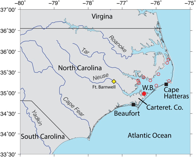
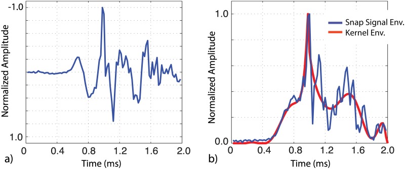
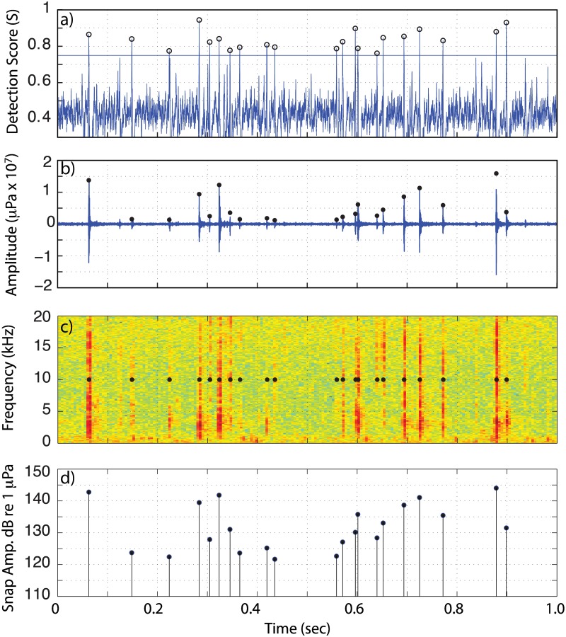
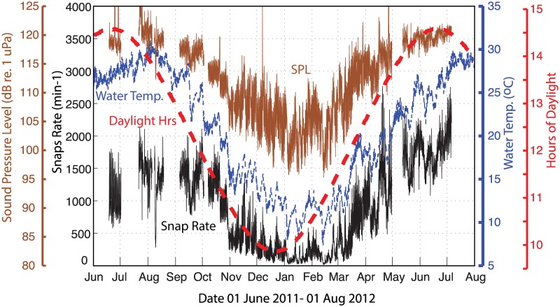
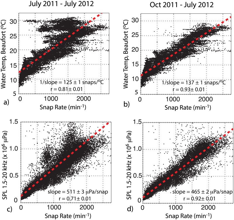
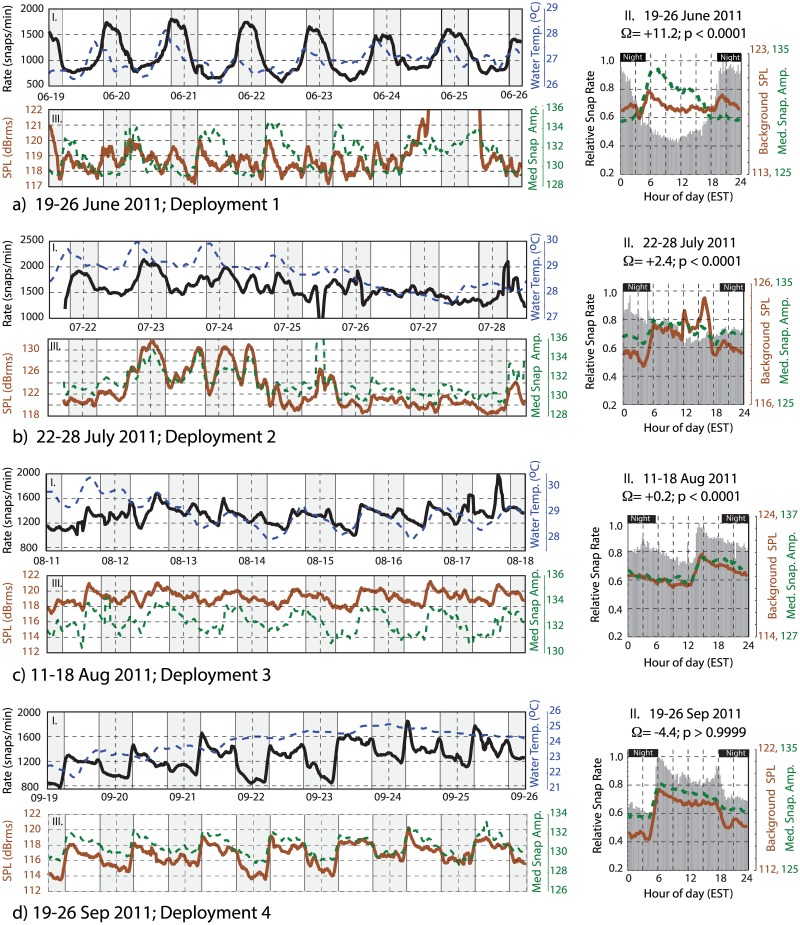
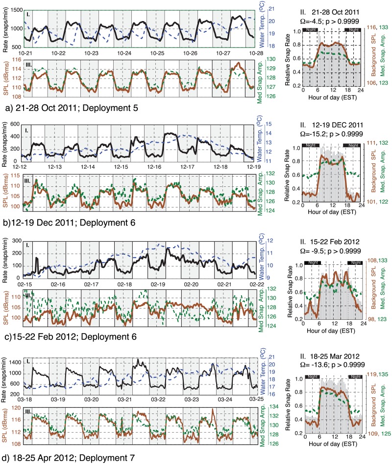
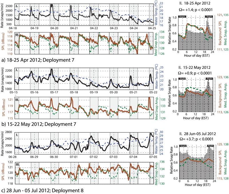
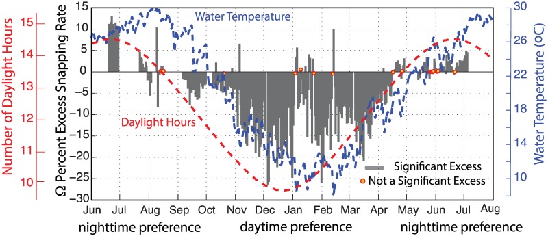
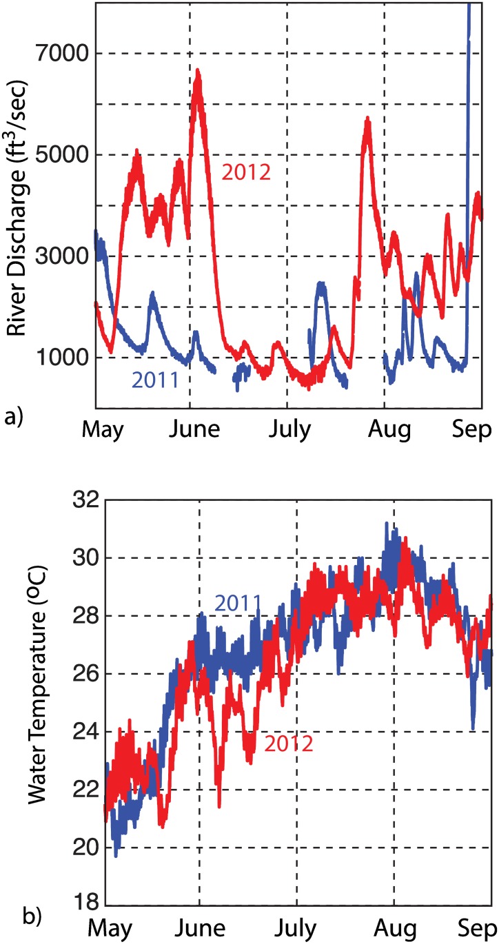
Ocean soundscapes convey important sensory information to marine life. Like many mid-to-low latitude coastal areas worldwide, the high-frequency (>1.5 kHz) soundscape of oyster reef habitat within the West Bay Marine Reserve (36°N, 76°W) is dominated by the impulsive, short-duration signals generated by snapping shrimp. Between June 2011 and July 2012, a single hydrophone deployed within West Bay was programmed to record 60 or 30 seconds of acoustic data every 15 or 30 minutes. Envelope correlation and amplitude information were then used to count shrimp snaps within these recordings. The observed snap rates vary from 1500-2000 snaps per minute during summer to <100 snaps per minute during winter. Sound pressure levels are positively correlated with snap rate (r = 0.71-0.92) and vary seasonally by ~15 decibels in the 1.5-20 kHz range. Snap rates are positively correlated with water temperatures (r = 0.81-0.93), as well as potentially influenced by climate-driven changes in water quality. Light availability modulates snap rate on diurnal time scales, with most days exhibiting a significant preference for either nighttime or daytime snapping, and many showing additional crepuscular increases. During mid-summer, the number of snaps occurring at night is 5-10% more than predicted by a random model; however, this pattern is reversed between August and April, with an excess of up to 25% more snaps recorded during the day in the mid-winter. Diurnal variability in sound pressure levels is largest in the mid-winter, when the overall rate of snapping is at its lowest, and the percentage difference between daytime and nighttime activity is at its highest. This work highlights our lack of knowledge regarding the ecology and acoustic behavior of one of the most dominant soniforous invertebrate species in coastal systems. It also underscores the necessity of long-duration, high-temporal-resolution sampling in efforts to understand the bioacoustics of animal behaviors and associated changes within the marine soundscape.

Fig 1. Location Map.

Oyster reserve sites in Pamlico Sound, North Carolina, USA (open red circles), including the West Bay Marine Reserve (solid red circle) that was acoustically monitored semi-continuously over the period between 18 June 2011 and 06 July 2012. Water temperature and atmospheric data are available from long-term NOAA monitoring sites in Beaufort and Cape Hatteras NC (black squares). Neuse River discharge data were collected near Fort Barnwell, NC (yellow triangle).

Fig 2. Snap detection using envelope correlation.

a) Band-pass filtered (1.5–20 kHz) waveform showing an individual snap. b) The envelope of the snap waveform (blue) and kernel (red). The detection score (correlation) between the signal envelope and kernel is 0.85, sufficient to declare detection.

Fig 3. Snap detection example.

An example of the detection score procedure applied to the West Bay acoustic data. Circles demote detections with a score S ≥ 0.75 and peak-to-peak amplitude ≥ 120 dB 1 μPa @ 1 m. a) detection score, b) pressure waveform, c) spectrogram, and d) peak-to-peak snap received level.

Fig 4. Snap rate vs. time.

The solid black line shows number of snaps detected per minute. The dashed blue line shows water temperature in °C from NOAA monitoring site near Beaufort, NC (Fig 1). Dashed red line shows the astronomical length of day in hours. Snap rate and sound pressure level information were smoothed using either a 7 (when recording Interval = 15 minutes) or 3 (when recording Interval = 30 minutes) point filter. Water temperature was interpreted at 15-minute intervals and smoothed using a 7-point filter.

Fig 5. Snap rate, SPL and water temperature correlations.

Panels (a) and (b) show the snap rate in West Bay vs. water temperatures measured at station (Beaufort, NC) for the periods July 2011-July 2012 and Oct 2011 –July 2012, respectively. Panels (c) and (d) show snap rate vs. root-mean-square sound pressure levels during these same periods. Red line shows least squares fit to the data. Slopes and correlation coefficients are shown in each panel; uncertainties are estimated using a bootstrap resampling.

Fig 6. Wavelet analysis.

Wavelet scalogram of the snap rate data generated using a Morlet wavelet. The black boxes delineate the 1-week duration time series examples shown in Figs 7–9. Unlike short-time Fourier techniques, the wavelet transform method makes use of variable length analysis windows and can often provide better temporal resolution than fixed-window-length spectral methods. The figure highlights the persistence, and varying strength, of the diurnal periodicity in snap count throughout the monitoring period. The snap rate time series intermittently exhibits additional variance at longer periods (2–4 days), which may be related to variations in water temperature (Fig 4) or water quality.

Fig 7. Time series examples June 2011- September 2011.

A series of one-week duration data windows are displayed. Date ranges and deployment numbers are shown for each example. Panels I and III show time series examples of snap rate (black), water temperature (dashed blue), 1.5–20 kHz band rms sound pressure level (brown), and median peak-to-peak snap amplitude (dashed green). All pressure data have units of dB re 1 μPa. The vertical scale is optimized for each week’s data to better visualize the patterns in panels I and III. The panels labeled II show weekly histogram plots of the relative number of snaps (black), along with the median sound pressure level (brown) and snap amplitude (dashed green) as a function of time of day. Black horizontal bars define nighttime periods. The vertical scale ranges are fixed for each panel II to represent the relative strength of the diurnal pattern from week-to-week. The percent excess within each of these weekly data windows is labeled. All time series are smoothed using either a 7 (when recording Interval = 15 minutes) or 3 (when recording Interval = 30 minutes) point filter. Time series example continued in Figs 8 and 9.

Fig 8. Time series examples October 2011- April 2012.

Panels I and III show time series examples of snap rate (black), water temperature (dashed blue), 1.5–20 kHz band rms sound pressure level (brown), and median peak-to-peak snap amplitude (dashed green). The panels labeled II show weekly histogram plots of the relative number of snaps (black), along with the median sound pressure level (brown) and snap amplitude (dashed green) as a function of time of day. See Fig 7 caption for additional information. Time series continued in Fig 9.

Fig 9. Time series examples April 2012- July 2012.

Panels I and III show time series examples of snap rate (black), water temperature (dashed blue), 1.5–20 kHz band rms sound pressure level (brown), and median peak-to-peak snap amplitude (dashed green). The panels labeled II show weekly histogram plots of the relative number of snaps (black), along with the median sound pressure level (brown) and snap amplitude (dashed green) as a function of time of day. See Fig 7 caption for additional information.

Fig 10. Diurnal snapping pattern.

Percent excess snap count throughout the 2011–2012 monitoring period within the West Bay Marine Reserve. Grey bars show the daily percent excess values that are statistically significant (95% confidence); circles denote days when small percent excess values are not significantly different. Positive percent excess indicates a preference for nighttime snapping; whereas, negative values indicate a preference for daytime snapping. The water temperature data from Beaufort NC are shown in blue, and the length of day in hours is shown red.

Fig 11. Inter-annual climate variability.

Environmental data from Pamlico Sound, NC during the summer of 2011 (blue) and 2012 (red). a) River discharge measured on the Neuse River near Fort Barnwell, NC (35.31°N, 77.30°W). b) Water temperature measured near Beaufort, NC.

References

1. Bormpoudakis D, Sueur J, Pantis JD. Spatial heterogeneity of ambient sound at the habitat type level: ecological implications and applications. Landscape Ecol. 2013;28: 495–506. 10.1007/s10980-013-9849-1 - DOI
1. Montgomery JC, Jeffs A, Simpson SD, Meekan M, Tindle C. Sound as an orientation cue for the pelagic larvae of reef fishes and Decapod Crustaceans. Advances in Marine Biology Elsevier. Volume 51; 2006. pp. 143–196. 10.1016/S0065-2881(06)51003-X - DOI - PubMed
1. Hughes AR, Mann DA, Kimbro DL. Predatory fish sounds can alter crab foraging behaviour and influence bivalve abundance. Proceedings of the Royal Society B: Biological Sciences. 2014;281: 20140715–20140715. 10.1098/rspb.2014.0715 - DOI - PMC - PubMed
1. Luczkovich JJ, Daniel HJ III, Hutchinson M, Jenkins T, Johnson SE, Pullinger RC, et al. Sounds of sex and death in the sea: Bottlenose Dolphin whistles suppress mating choruses of Silver Perch. Bioacoustics. 2000;10: 323–334. 10.1080/09524622.2000.9753441 - DOI
1. Cato DH, Noad M, McCauley RD. Passive acoustics as a key to the study of marine animals Sounds in the sea: From ocean acoustics to acoustical oceanography. Cambridge MA; 2005. pp. 411–429.
Publication types
LinkOut - more resources