Model-Based Geostatistical Mapping of the Prevalence of Onchocerca volvulus in West Africa

Abstract

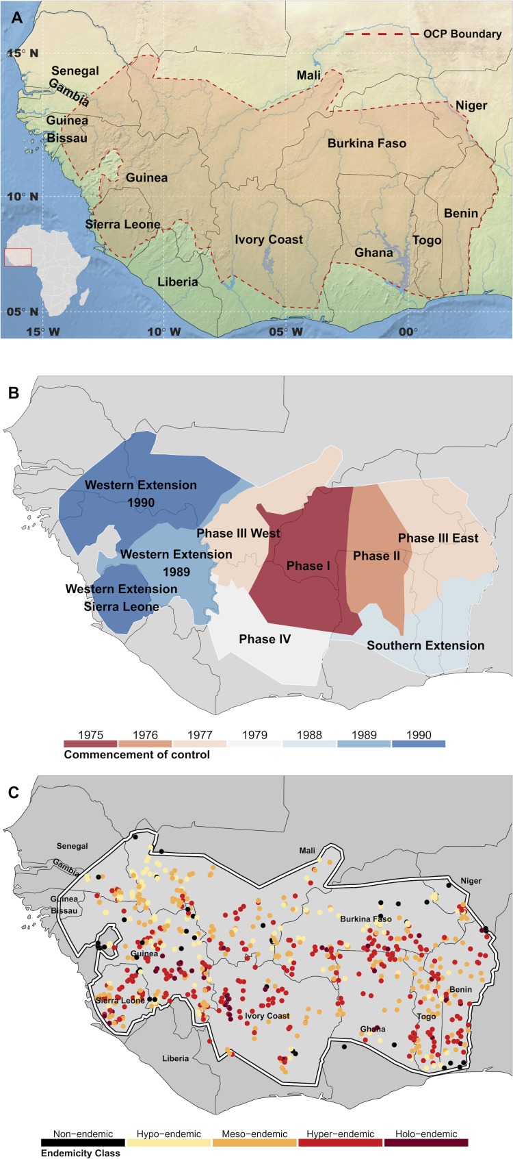
Background: The initial endemicity (pre-control prevalence) of onchocerciasis has been shown to be an important determinant of the feasibility of elimination by mass ivermectin distribution. We present the first geostatistical map of microfilarial prevalence in the former Onchocerciasis Control Programme in West Africa (OCP) before commencement of antivectorial and antiparasitic interventions.

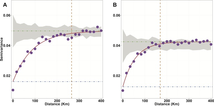
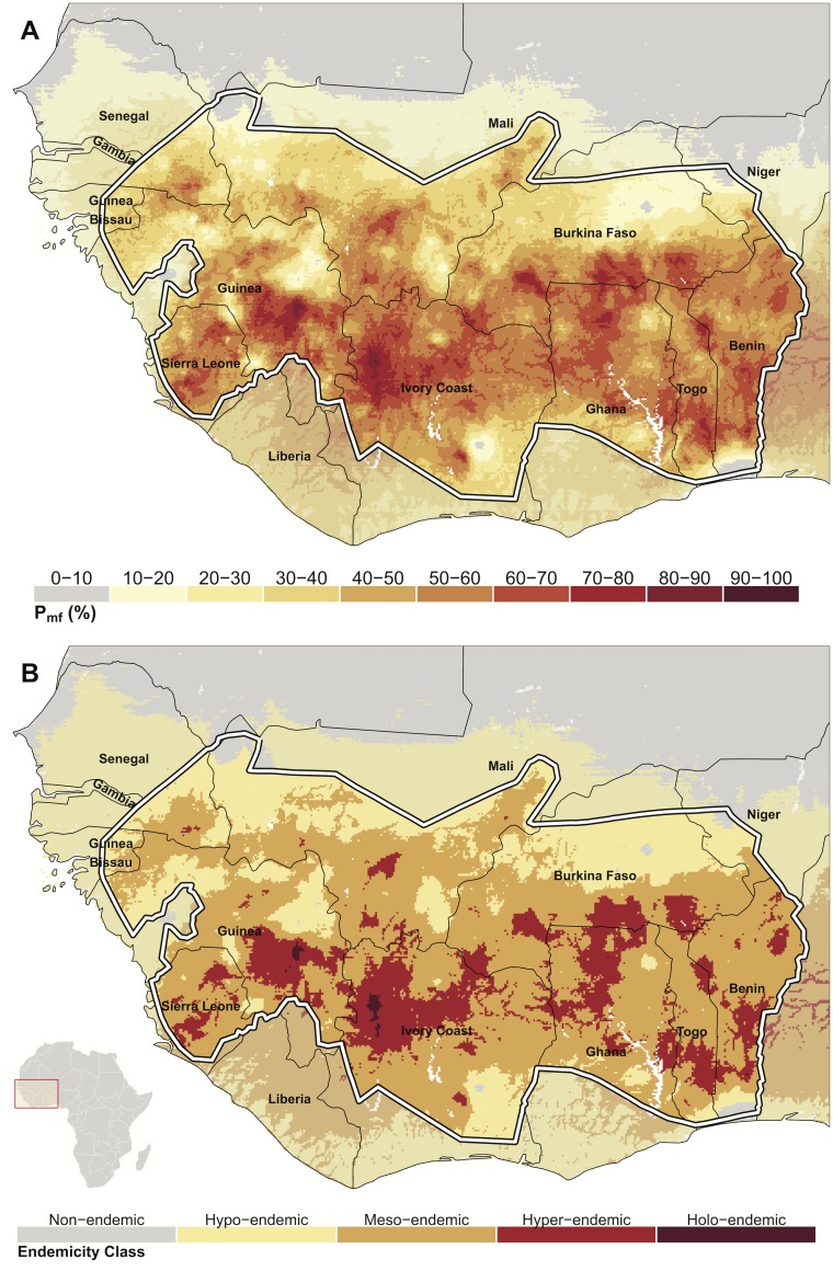
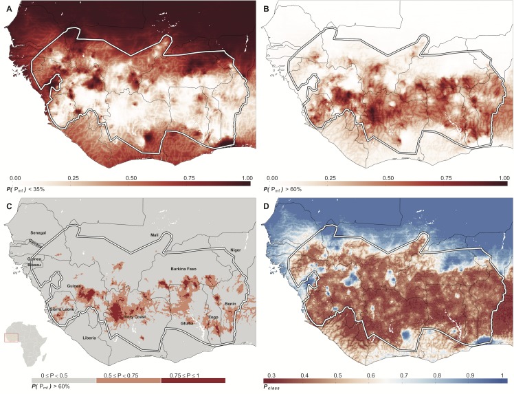
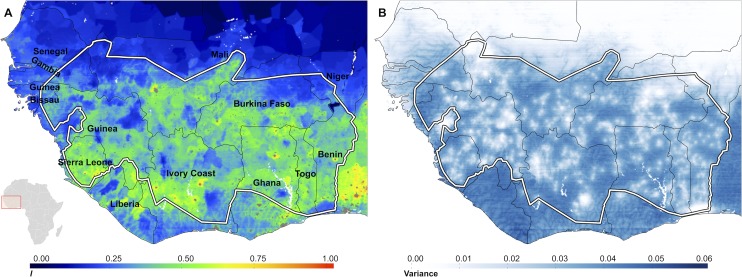
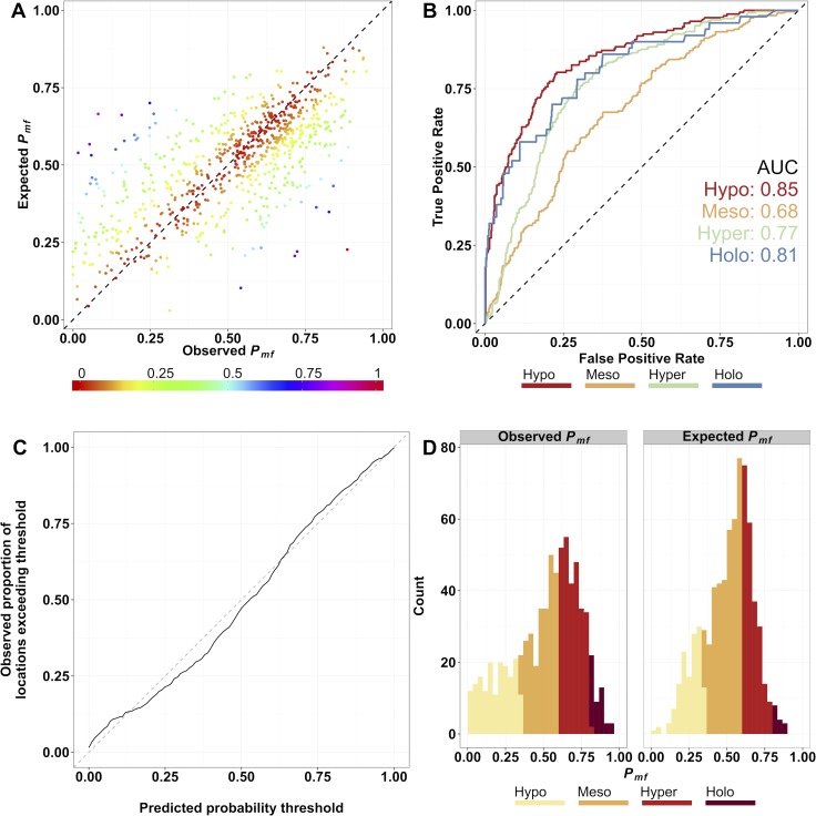
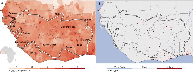
Methods and findings: Pre-control microfilarial prevalence data from 737 villages across the 11 constituent countries in the OCP epidemiological database were used as ground-truth data. These 737 data points, plus a set of statistically selected environmental covariates, were used in a Bayesian model-based geostatistical (B-MBG) approach to generate a continuous surface (at pixel resolution of 5 km x 5km) of microfilarial prevalence in West Africa prior to the commencement of the OCP. Uncertainty in model predictions was measured using a suite of validation statistics, performed on bootstrap samples of held-out validation data. The mean Pearson's correlation between observed and estimated prevalence at validation locations was 0.693; the mean prediction error (average difference between observed and estimated values) was 0.77%, and the mean absolute prediction error (average magnitude of difference between observed and estimated values) was 12.2%. Within OCP boundaries, 17.8 million people were deemed to have been at risk, 7.55 million to have been infected, and mean microfilarial prevalence to have been 45% (range: 2-90%) in 1975.

Conclusions and significance: This is the first map of initial onchocerciasis prevalence in West Africa using B-MBG. Important environmental predictors of infection prevalence were identified and used in a model out-performing those without spatial random effects or environmental covariates. Results may be compared with recent epidemiological mapping efforts to find areas of persisting transmission. These methods may be extended to areas where data are sparse, and may be used to help inform the feasibility of elimination with current and novel tools.

Fig 1. Maps of the Onchocerciasis Control Programme area.

A) Map showing the area covered by the Onchocerciasis Control Programme (OCP) in West Africa. The red dashed line delineates the limit of anti-vectorial and/or anti-parasitic activities carried out by the OCP between 1975 and 2002. B) Map of the operational phases of the OCP. Until 1987 the method of control was almost exclusively anti-vectorial, through larviciding of vector breeding habitats. From 1987 ivermectin was used extensively, and almost exclusively in the Western Extension zones. C) Locations of the village surveys which met the criteria for inclusion in this study. A total of 737 survey sites were selected, from 5,817 surveys. The survey data displayed are coloured by endemicity class of crude microfilarial prevalence in the population aged ≥5 years. For the cut-off values of microfilarial prevalence corresponding to each endemicity category see Main Text and legend of Fig 3B.

Fig 2. Semi-variogram analysis of spatial trend in the data.

A) Empirical variogram assuming a constant mean trend across the study region (i.e. without the use of environmental covariates). B) The spatial trend present in the data after accounting for the effects of explanatory environmental covariates by incorporating a spatially-varying mean trend surface. The purple dots are the mean semivariance values between all pairs of villages with separation distance contained within a discrete distance bin, with the mid point of each bin used to locate the dots on the x-axis. The red solid line is the fitted theoretical variogram model. The dash-dot blue horizontal lines represent the nugget variance τ², encompassing sources of non-spatial variation. The dash-dot green horizontal lines represent the sill variance, σ², which is the estimated variance of the spatial process S(⋅). The dashed orange vertical lines are the range at which the variance asymptotically reaches 95% of its sill value and is given by −ln(0.05)ϕ, where ϕ is the range parameter. Beyond this value the covariance between locations does not significantly depend on separation distance. The grey shaded areas are the Monte Carlo envelopes of variance expected by chance, obtained by randomly reassigning the values of microfilarial prevalence at data locations and calculating the empirical semivariogram. The empirical variogram (A) mostly lies outside this region and, therefore, there is therefore a significant spatial trend present in the data. The trend in semivariogram (B) is fitted to the residuals resulting after adjusting for the set of linear predictors of the environmental covariate model. The reduction in range parameter, compared to the mean trend shows that the environmental covariates account for some (but not all) of the observed spatial variation. As some of such variation still lies outside of the Monte-Carlo envelope of spatially random data, there is still a significant spatial trend.

Fig 3. The spatial distribution of onchocerciasis microfilarial prevalence in West Africa.

A) The mean of the predictive posterior distribution of microfilarial prevalence in the population aged ≥ 5 years (P_mf) for each pixel in the study area. There are no pseudo-absence data points in this model (i.e., pragmatically-generated points of zero-prevalence in areas of known absence of disease) and, therefore, the grey areas in the north of the map, where predictions of prevalence are very low, are entirely determined by the value of the environmental covariates (the closest villages are too distal to exert a spatial effect). The white boundary denotes the limits of the OCP area. B) Endemicity class classifications for the mean of the predictive posterior, based on a modification of the OCP endemicity categories. Areas where prevalence is very low are shown by sub-dividing the hypoendemic class into two categories, a non-endemic/sporadic endemicity class, where microfilarial prevalence is <10%, and a hypoendemic class where prevalence ≥10% but <35%. Other categories are mesoendemic: ≥35% and < 60%; hyperendemic: ≥ 60% and < 80%, and highly hyperendemic (or holoendemic): ≥ 80%.

Fig 4. Predictive inference for threshold exceedance and endemicity class membership.

A) The posterior predictive probability that microfilarial prevalence for each map pixel is less than 35%. The model output is mapped on a continuous scale from 0 to 1, with dark red representing a high degree of certainty that prevalence does not exceed the threshold of 35%. B) The continuous posterior predictive probability that microfilarial prevalence exceeds the threshold for hyperendemicity of 60%. C) Model output as in Fig 4B but categorised into broad probability intervals. Maps of this nature may have utility for the optimal targeting of current and novel control interventions by programme managers. Light-grey areas are pixels with a probability < 50% of exceeding the 60% threshold; pink pixels denote that the probability of exceeding hyperendemicity lies between 50% and 75%; deep-red colours represent a probability > 75% of exceeding this threshold. D) The probability of each map pixel being in the endemicity class to which it was assigned (Ρ_class). With 4 endemicity classes the probability ranges from a minimum of 0.25 to 1, with a value of one meaning that all realisations from the predictive posterior were assigned to the same endemicity class. In all panels the red boundary denotes the OCP limits.

Fig 5. Maps of uncertainty in predictive posterior realisations.

A) The population weighted index of uncertainty is calculated as in [61] and is a pragmatic representation of how important uncertainty in the predictive posteriors is likely to be. The uncertainty index is calculated by taking the log₁₀(pop₇₅ +1)×1/P_class where pop₇₅ is the population count for 1975 and Ρ_class is the probability of endemicity class assignment (Fig 4D). B) Map of the variance of predictive posteriors. Higher values mean more diffuse posterior distributions and hence greater uncertainty in model estimates. The lowest uncertainty is found in pixels proximal to data locations. In both panels the red boundary denotes the OCP limits.

Fig 6. Plots of model performance.

A) Scatter-plot of observed versus estimated microfilarial prevalence in those aged ≥ 5 years (P_mf) at validation locations. The Pearson’s correlation coefficient between observed and estimated values was 0.693. The 1:1 line of perfect correlation is shown for reference. The data are coloured by the absolute difference between observed and expected values, mapped from a continuum between 0 and 1. B) Receiver Operating Characteristic (ROC) curves for each endemicity class (black line, hypoendemic; red line, mesoendemic; green line, hyperendemic; blue line, holoendemic). AUC values for each endemicity class are also displayed on the plot. C) Probability-probability plot of the proportion of true values of P_mf at validation locations that exceed their predicted probability threshold for a series of probability thresholds from 1% to 100%. Deviation from the 1:1 dashed line in this plot represents the difference between the distributions of observed and estimated microfilarial prevalence values at validation locations. D) Frequency histogram of observed and estimated P_mf at validation locations, classified according to their true class (Observed P_mf panel) and estimated endemicity class (Expected P_mf panel).

Fig 7. Estimated gridded population counts for 1975 and urban extents mask.

A) Each map pixel contains the log₁₀ transformed count of the total population +1 (to avoid negative values for population counts), aged ≥ 5 years estimated to live in that map pixel in 1975. Summing pixels by country, the totals show < 0.8% difference to the United Nations World Population Prospects (2012 Revision) country census figures for 1975. B) Red pixels delineate pixels that are classified as urban extents according the Global Rural-Urban Mapping Project (GRUMP V1.0). Estimates in urban pixels and water bodies do not count towards the population totals of numbers infected shown in Table 4. In both panels the white boundary denotes the OCP limits.

References

1. London Declaration on Neglected Tropical Diseases. Uniting to combat neglected tropical diseases: Ending the neglect and reaching 2020 goals. 2012. [http://unitingtocombatntds.org/sites/default/files/resource_file/london_...]. Accessed 30 November 2015.
1. World Health Organization. Accelerating work to overcome the global impact of neglected tropical diseases–A roadmap for implementation. 2012. [http://www.who.int/neglected_diseases/NTD_RoadMap_2012_Fullversion.pdf]. Accessed 30 November 2015.
1. Kim YE, Remme JH, Steinmann P, Stolk WA, Roungou JB, Tediosi F. Control, elimination, and eradication of river blindness: scenarios, timelines, and ivermectin treatment needs in Africa. PLoS Negl Trop Dis. 2015;9(4): e0003664 (Correction in PLoS Negl Trop Dis. 2015;9(5): e0003777). 10.1371/journal.pntd.0003664 - DOI - PMC - PubMed
1. Bradley JE, Whitworth J, Basáñez MG. Onchocerciasis In: Wakelin D, Cox F, Despommier D, Gillespie, editors. Topley and Wilson’s Microbiology and Microbial Infections. Volume Parasitology. 10th edition London: Hodder Arnold; 2005. pp: 781–801.
1. Murdoch ME, Hay RJ, Mackenzie CD, Williams JF, Ghalib HW, Cousens S, et al. A clinical classification and grading system of the cutaneous changes in onchocerciasis. Br J Dermatol. 1993;129(3): 260–269. - PubMed
Publication types